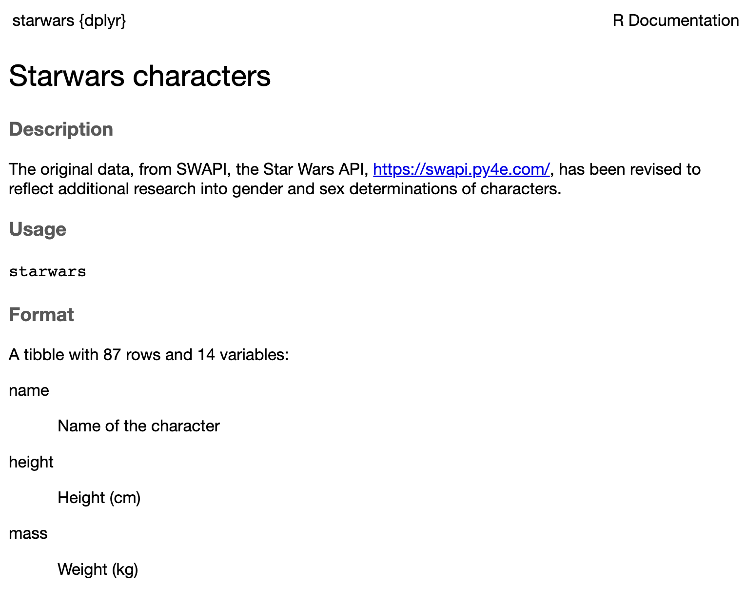
Visualizing data

Data visualization and transformation

Data Science with R

What is in a dataset?

Dataset terminology

• Each row is an observation
• Each column is a variable

starwars

# A tibble: 87 × 14
   name         height  mass hair_color skin_color eye_color
   <chr>         <int> <dbl> <chr>      <chr>      <chr>    
 1 Luke Skywal…    172    77 blond      fair       blue     
 2 C-3PO           167    75 <NA>       gold       yellow   
 3 R2-D2            96    32 <NA>       white, bl… red      
 4 Darth Vader     202   136 none       white      yellow   
 5 Leia Organa     150    49 brown      light      brown    
 6 Owen Lars       178   120 brown, gr… light      blue     
 7 Beru Whites…    165    75 brown      light      blue     
 8 R5-D4            97    32 <NA>       white, red red      
 9 Biggs Darkl…    183    84 black      light      brown    
10 Obi-Wan Ken…    182    77 auburn, w… fair       blue-gray
# ℹ 77 more rows
# ℹ 8 more variables: birth_year <dbl>, sex <chr>,
#   gender <chr>, homeworld <chr>, species <chr>,
#   films <list>, vehicles <list>, starships <list>

Luke Skywalker

What’s in the Star Wars data?

Take a glimpse() at the data:

glimpse(starwars)

Rows: 87
Columns: 14
$ name       <chr> "Luke Skywalker", "C-3PO", "R2-D2", "Da…
$ height     <int> 172, 167, 96, 202, 150, 178, 165, 97, 1…
$ mass       <dbl> 77, 75, 32, 136, 49, 120, 75, 32, 84, 7…
$ hair_color <chr> "blond", NA, NA, "none", "brown", "brow…
$ skin_color <chr> "fair", "gold", "white, blue", "white",…
$ eye_color  <chr> "blue", "yellow", "red", "yellow", "bro…
$ birth_year <dbl> 19.0, 112.0, 33.0, 41.9, 19.0, 52.0, 47…
$ sex        <chr> "male", "none", "none", "male", "female…
$ gender     <chr> "masculine", "masculine", "masculine", …
$ homeworld  <chr> "Tatooine", "Tatooine", "Naboo", "Tatoo…
$ species    <chr> "Human", "Droid", "Droid", "Human", "Hu…
$ films      <list> <"A New Hope", "The Empire Strikes Bac…
$ vehicles   <list> <"Snowspeeder", "Imperial Speeder Bike…
$ starships  <list> <"X-wing", "Imperial shuttle">, <>, <>…

Get to know the data

How many rows and columns does this dataset have? What does each row represent? What does each column represent?

?starwars

Dimensions of the data

How many rows and columns does this dataset have?

nrow(starwars) # number of rows

[1] 87

ncol(starwars) # number of columns

[1] 14

dim(starwars)  # dimensions (row column)

[1] 87 14

Exploratory data analysis

What is EDA?

Exploratory data analysis (EDA) is an approach for analyzing data sets to summarize their main characteristics:

• Visualize – this is what we’ll focus on first
• Summarize - this is what we’ll focus on next
• Both of these may require data wrangling, manipulation, transformation at (or before) this stage of the analysis

Mass vs. height

How would you describe the relationship between mass and height of Star Wars characters? What other variables would help us understand data points that don’t follow the overall trend? Who is the not so tall but really chubby character?

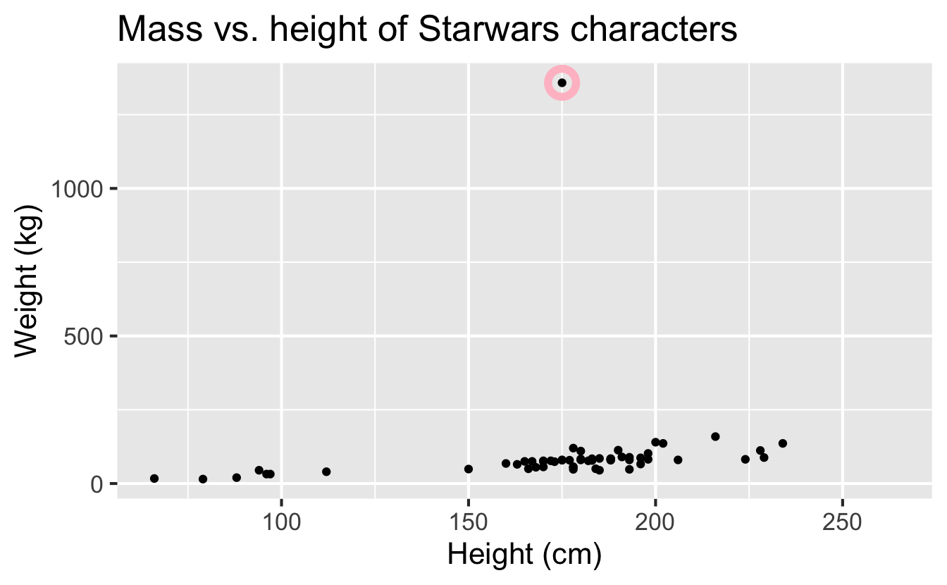
Jabba!

Data visualization

“The simple graph has brought more information to the data analyst’s mind than any other device.” — John Tukey

• Data visualization, an important part of exploratory data analysis, is the creation and study of the visual representation of data
• Many tools for visualizing data – R is one of them
• Many approaches/systems within R for making data visualizations – ggplot2 is one of them, and that’s what we’re going to use

Why visualize?

Anscombe’s quartet

library(Tmisc)
quartet

   set  x     y
1    I 10  8.04
2    I  8  6.95
3    I 13  7.58
4    I  9  8.81
5    I 11  8.33
6    I 14  9.96
7    I  6  7.24
8    I  4  4.26
9    I 12 10.84
10   I  7  4.82
11   I  5  5.68
12  II 10  9.14
13  II  8  8.14
14  II 13  8.74
15  II  9  8.77
16  II 11  9.26
17  II 14  8.10
18  II  6  6.13
19  II  4  3.10
20  II 12  9.13
21  II  7  7.26
22  II  5  4.74
23 III 10  7.46
24 III  8  6.77
25 III 13 12.74
26 III  9  7.11
27 III 11  7.81
28 III 14  8.84
29 III  6  6.08
30 III  4  5.39
31 III 12  8.15
32 III  7  6.42
33 III  5  5.73
34  IV  8  6.58
35  IV  8  5.76
36  IV  8  7.71
37  IV  8  8.84
38  IV  8  8.47
39  IV  8  7.04
40  IV  8  5.25
41  IV 19 12.50
42  IV  8  5.56
43  IV  8  7.91
44  IV  8  6.89

Summarizing Anscombe’s quartet

quartet |>
  group_by(set) |>
  summarise(
    mean_x = mean(x), 
    mean_y = mean(y),
    sd_x = sd(x),
    sd_y = sd(y),
    r = cor(x, y)
  )

# A tibble: 4 × 6
  set   mean_x mean_y  sd_x  sd_y     r
  <fct>  <dbl>  <dbl> <dbl> <dbl> <dbl>
1 I          9   7.50  3.32  2.03 0.816
2 II         9   7.50  3.32  2.03 0.816
3 III        9   7.5   3.32  2.03 0.816
4 IV         9   7.50  3.32  2.03 0.817

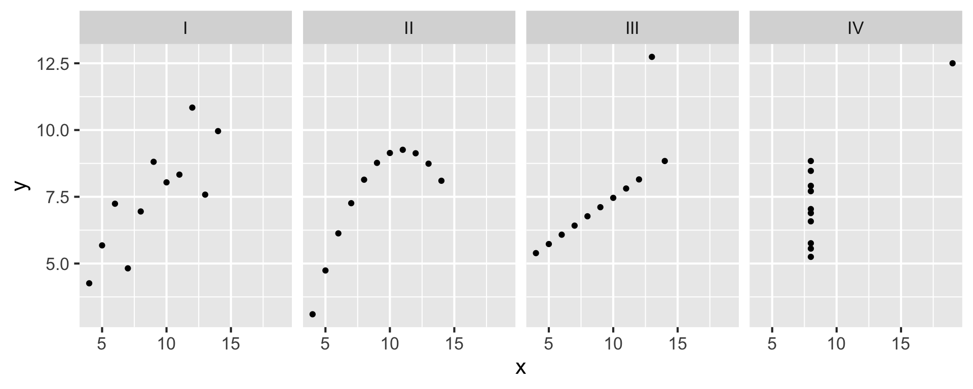
Visualizing Anscombe’s quartet

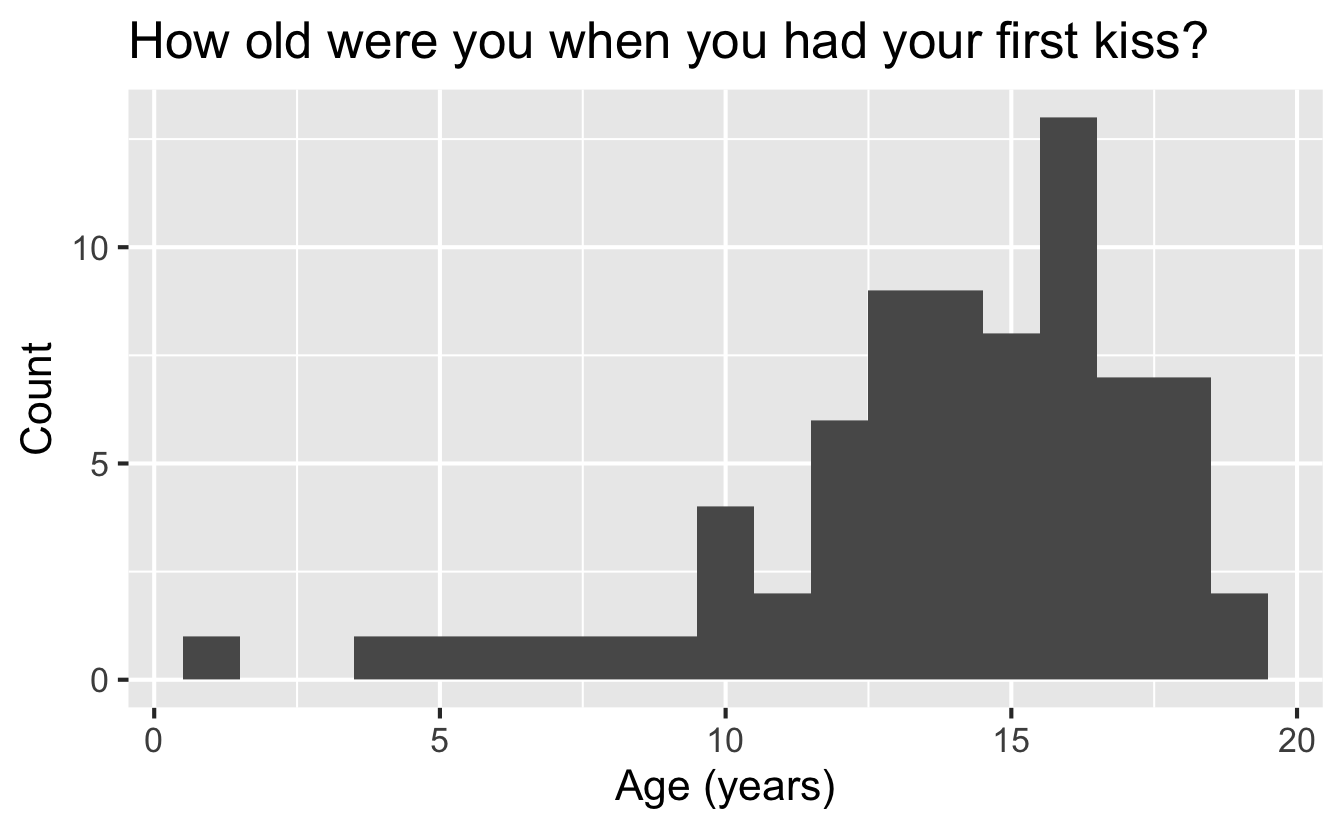
ggplot(quartet, aes(x = x, y = y)) +
  geom_point() +
  facet_wrap(~ set, ncol = 4)

Age at first kiss

A group of college students were asked “How old were you when you had your first kiss?” on a survey. First, think about how you might expect the distribution of their responses to look.

Then, examine the plot below. Do you see anything out of the ordinary?

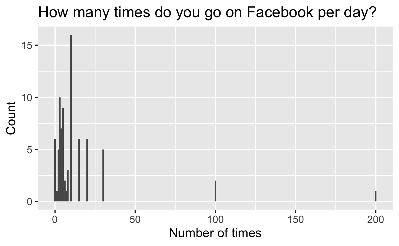
Facebook visits

Same group of college students were also asked “How many times do you go on Facebook per day?” First, think about how you might expect the distribution of their responses to look.

Then, examine the plot below. How are people reporting lower vs. higher values of FB visits?