Grammar of graphics

Data visualization and transformation

Data Science with R

Grammar of graphics

Grammar of Graphics

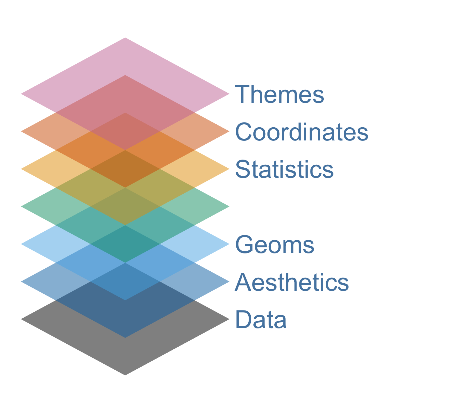
• The grammar of graphics is a tool that enables us to concisely describe the components of a graphic
• The ggplot2 package, which is part of tidyverse, implements the grammar of graphics in R

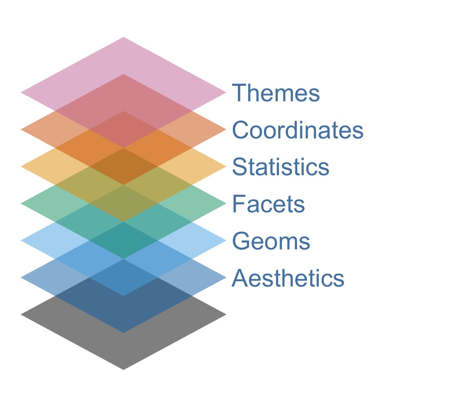
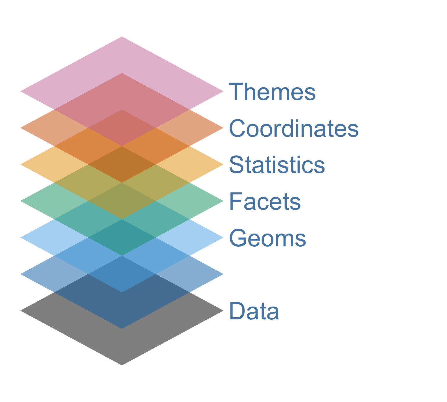
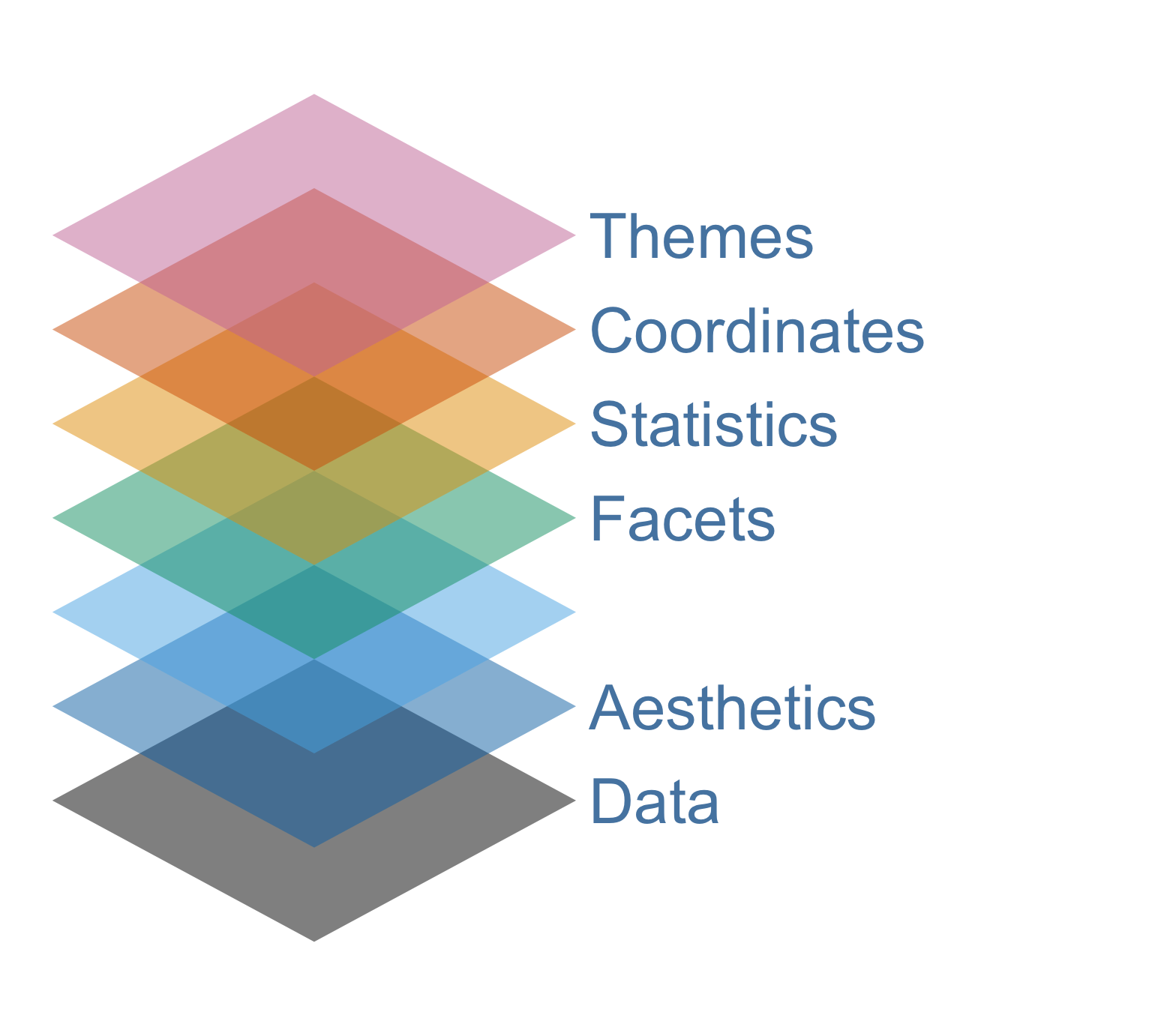
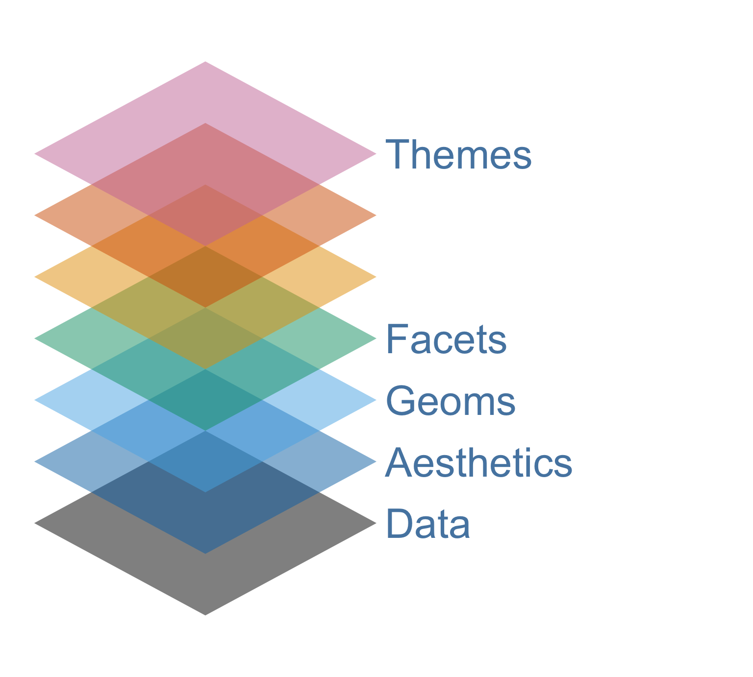
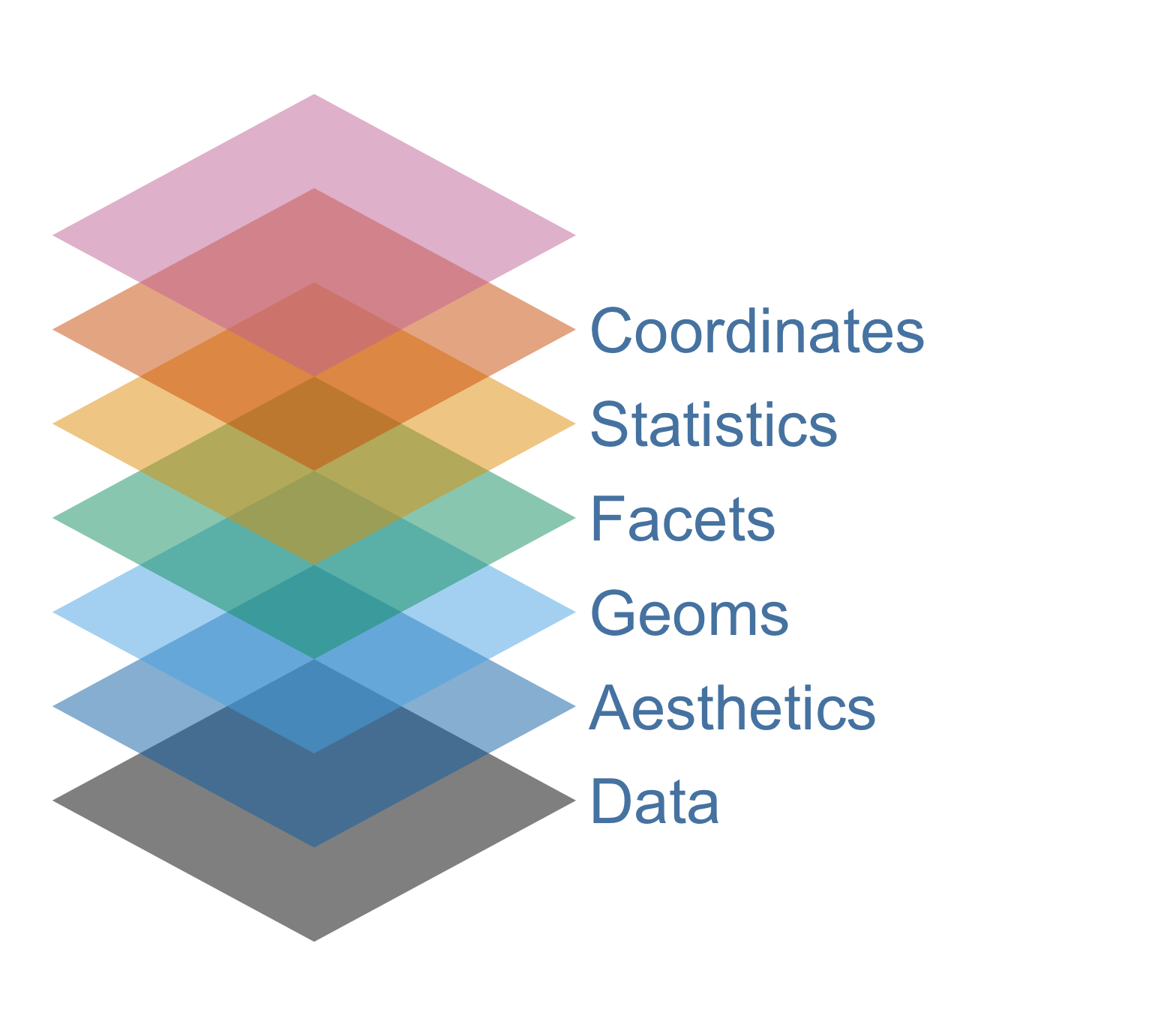
Layers

With ggplot2, you can create a wide variety of plots layer-by-layer:

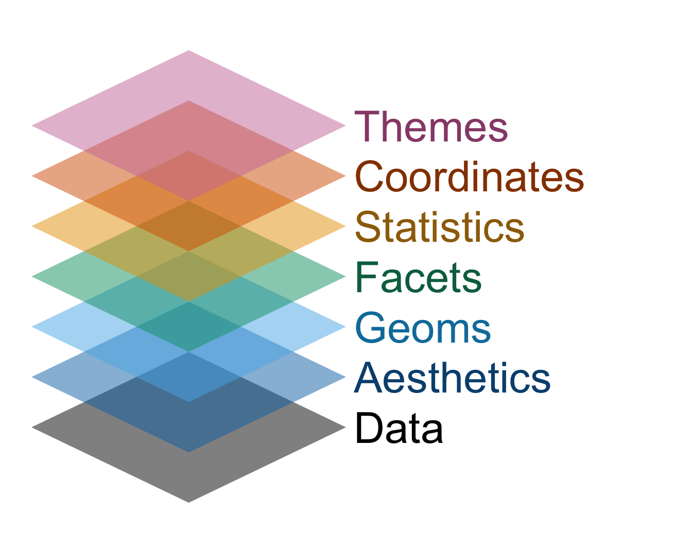
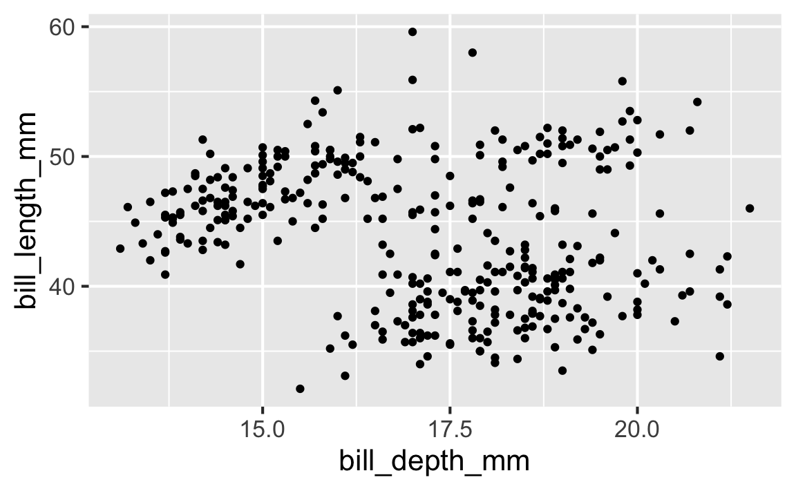
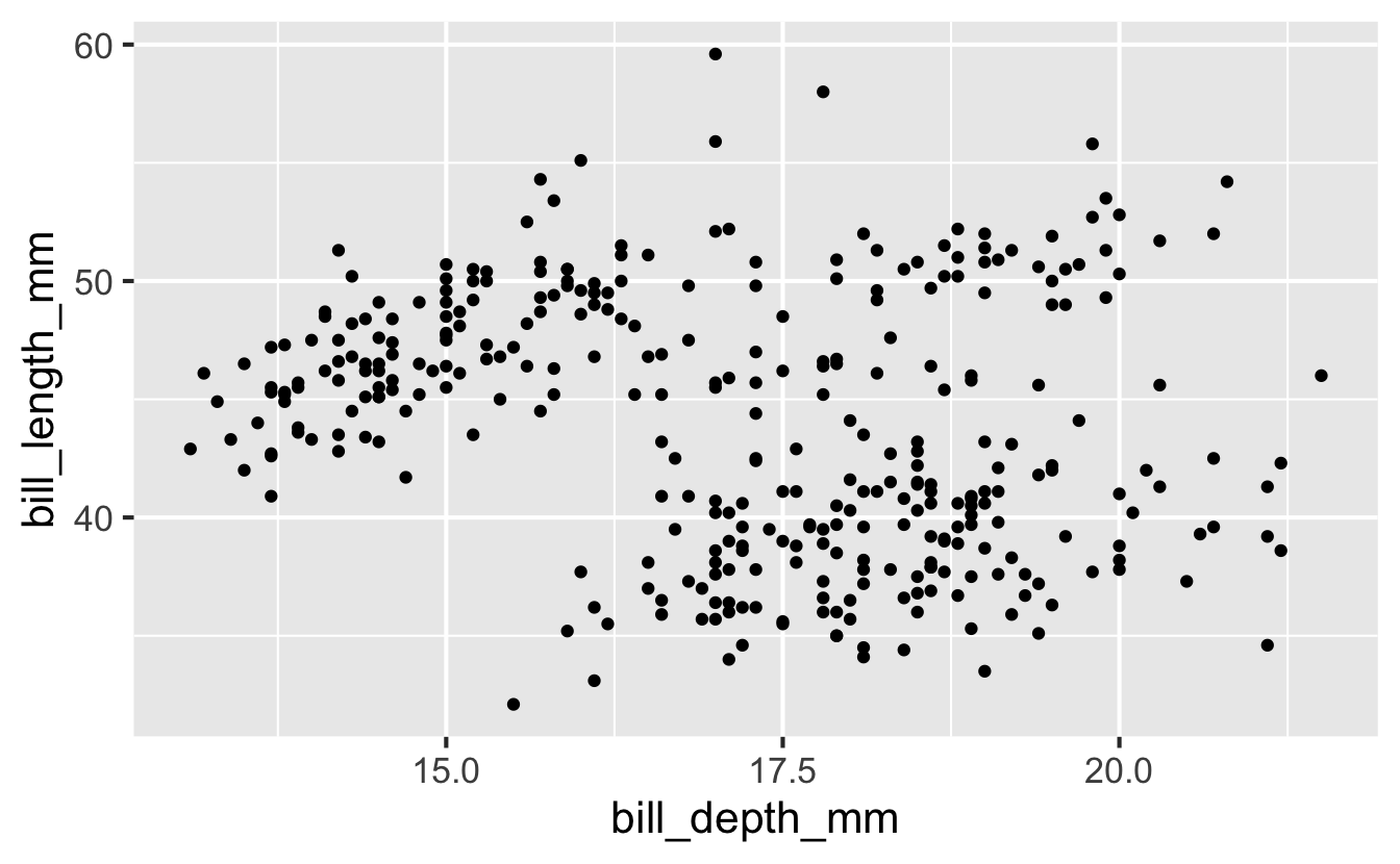
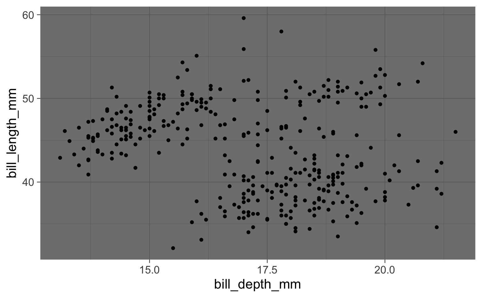
Layer 1: Data

Data

Foundation of the plot that gives you the canvas on which you can “paint” your data:

ggplot(penguins)

Layer 2: Aesthetics

Aesthetics

Characteristics of plotting characters that can be mapped to a specific variable in the data, e.g.:

• color
• shape
• size
• alpha (transparency)
• …

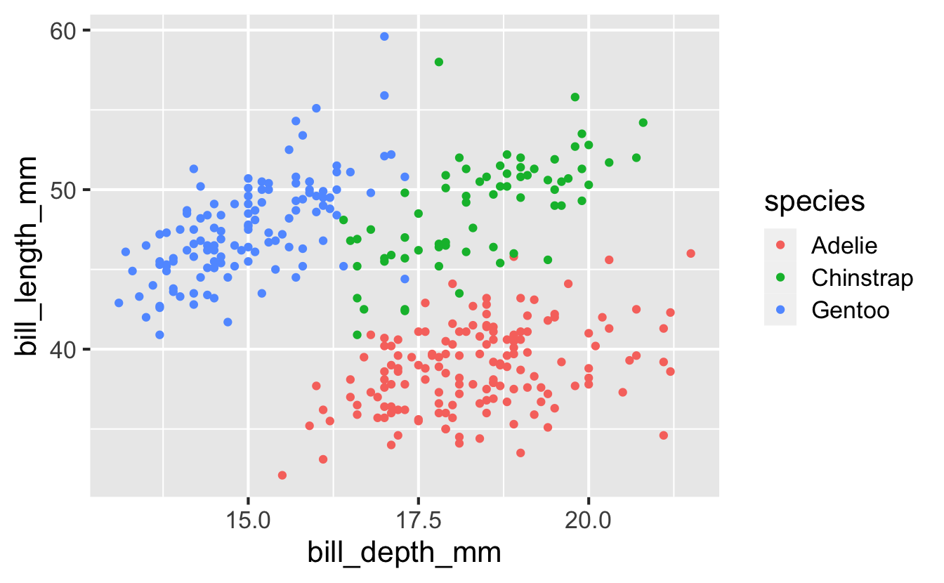
Color

The color aesthetic mapped to species:

ggplot(
  penguins,
  aes(
    x = bill_depth_mm, 
    y = bill_length_mm,
    color = species
    )
  ) +
  geom_point()

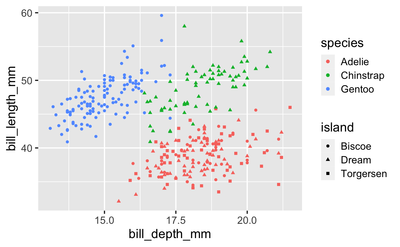
Shape

The shape aesthetic mapped to island:

ggplot(
  penguins,
  aes(
    x = bill_depth_mm, 
    y = bill_length_mm,
    color = species,
    shape = island
    )
  ) +
  geom_point()

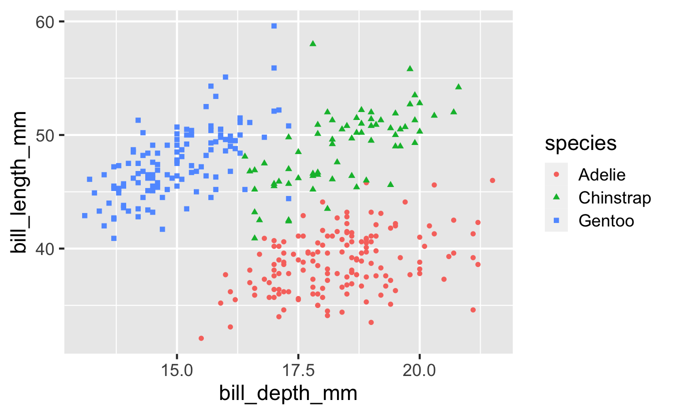
Color and shape

The color and shape aesthetics mapped to species:

ggplot(
  penguins,
  aes(
    x = bill_depth_mm, 
    y = bill_length_mm,
    color = species,
    shape = species
    )
  ) +
  geom_point()

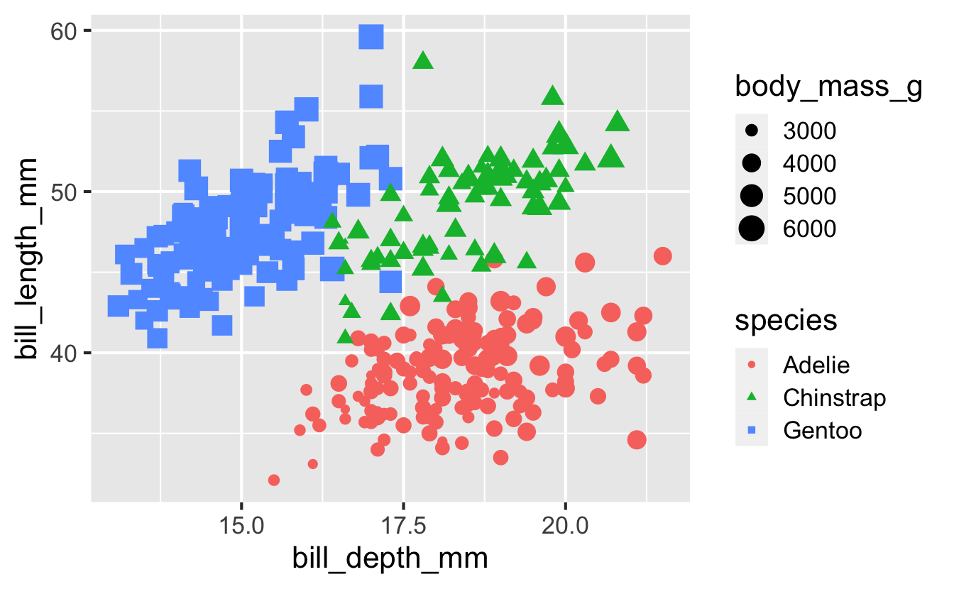
Size

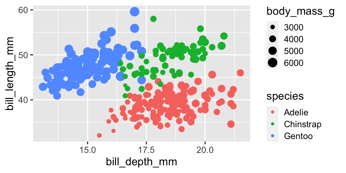
The size aesthetic mapped to body_mass_g:

ggplot(
  penguins,
  aes(
    x = bill_depth_mm, 
    y = bill_length_mm,
    color = species,
    shape = species,
    size = body_mass_g
    )
  ) +
  geom_point()

Alpha

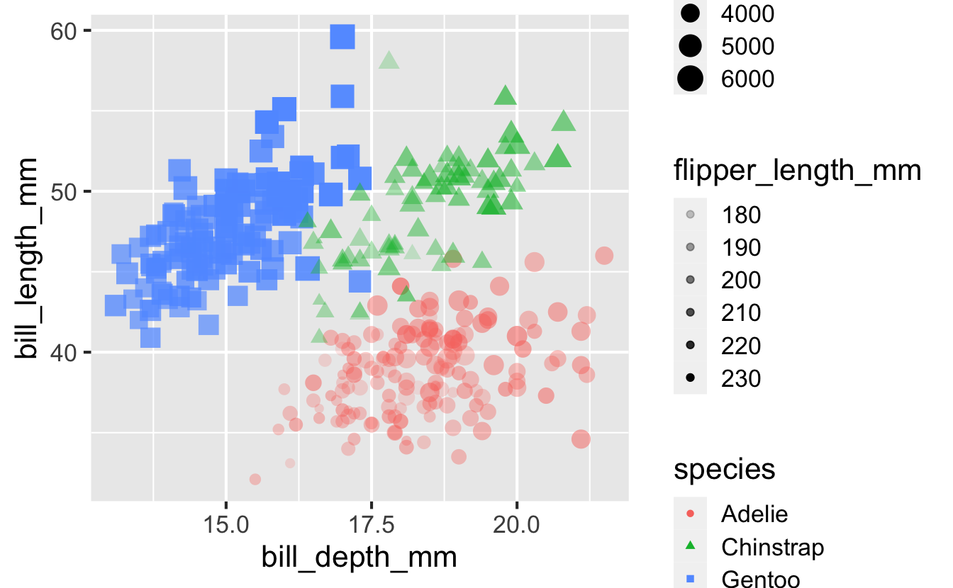
The alpha aesthetic mapped to flipper_length_mm:

ggplot(
  penguins,
  aes(
    x = bill_depth_mm, 
    y = bill_length_mm,
    color = species,
    shape = species,
    size = body_mass_g,
    alpha = flipper_length_mm
    )
  ) +
  geom_point()

Mapping vs. setting

Mapping:

ggplot(
  penguins,
  aes(
    x = bill_depth_mm, y = bill_length_mm,
    color = species,
    size = body_mass_g
    )
  ) + 
  geom_point()

Setting:

ggplot(
  penguins,
  aes(
    x = bill_depth_mm, y = bill_length_mm
    )
  ) + 
  geom_point(
    color = "red",
    size = 3
  )

Mapping vs. setting

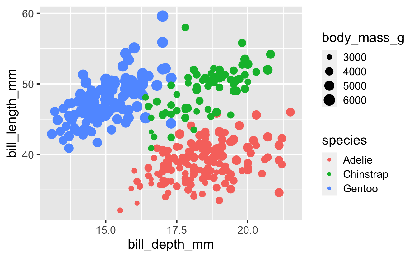
Mapping:

Determine the size, alpha, etc. of points based on the values of a variable in the data – goes into aes():

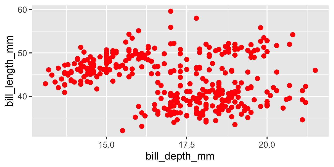
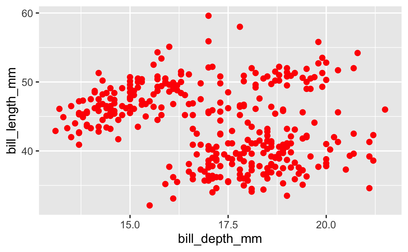
Setting:

Determine the size, alpha, etc. of points not based on the values of a variable in the data – goes into geom_*():

Layer 3: Geoms

Geoms

Visual representations of data points:

• Short for geometric objects
• geom_*() functions are used to add geoms to a plot
• Each geom adds a layer to the plot

geom_point()

ggplot(
  penguins, 
  aes(x = bill_depth_mm, y = bill_length_mm)
  ) + 
  geom_point()

geom_smooth()

ggplot(
  penguins,
  aes(x = bill_depth_mm, y = bill_length_mm)
  ) + 
  geom_point() +
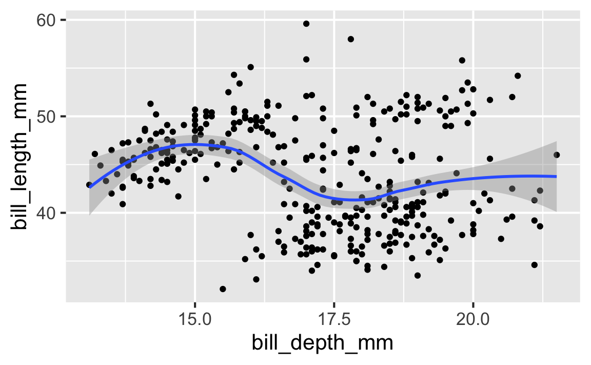
  geom_smooth()

and many more soon…

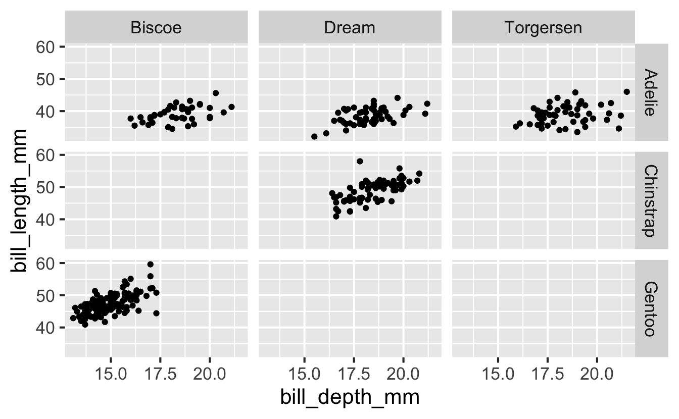
Layer 4: Facets

Faceting - what and why

• Smaller plots that each display different subsets of the data
• Also referred to as small multiples
• Useful for exploring conditional relationships and large data

Faceting - how

ggplot(
  penguins, 
  aes(
    x = bill_depth_mm, 
    y = bill_length_mm)
  ) + 
  geom_point()

Faceting - how

ggplot(
  penguins, 
  aes(
    x = bill_depth_mm, 
    y = bill_length_mm)
  ) + 
  geom_point() +
  facet_grid(species ~ island)

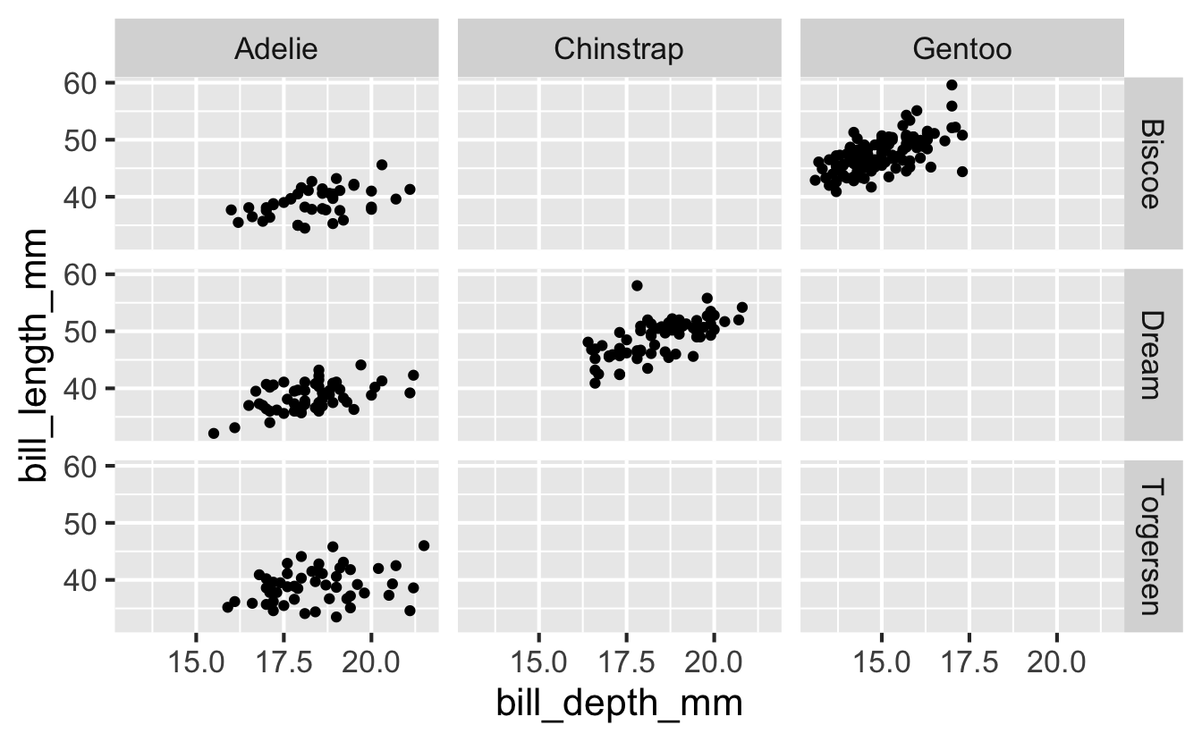
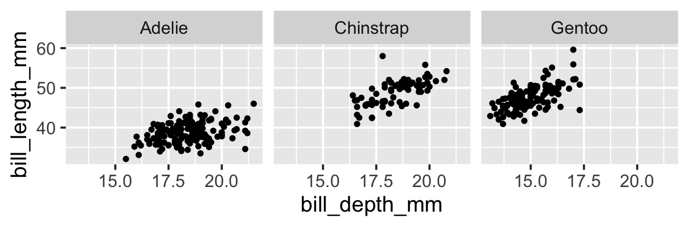
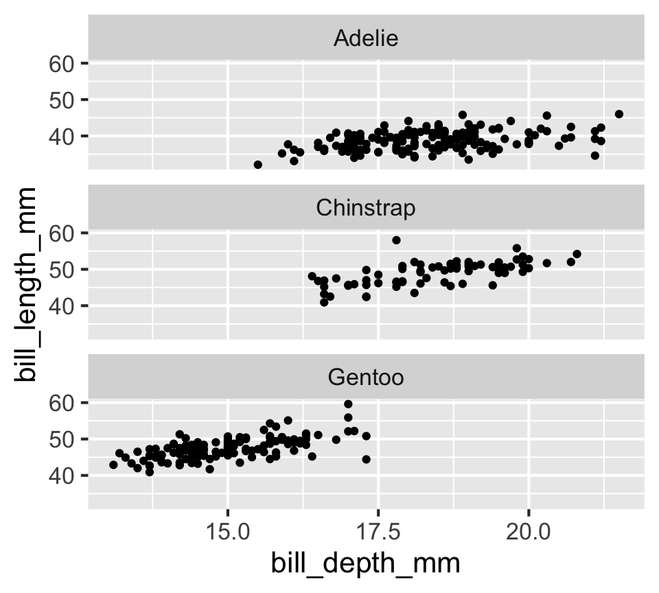
Faceting by two variables

species on rows, island on columns:

ggplot(penguins, aes(x = bill_depth_mm, y = bill_length_mm)) + 
  geom_point() +
  facet_grid(species ~ island)

island on rows, species on columns:

ggplot(penguins, aes(x = bill_depth_mm, y = bill_length_mm)) + 
  geom_point() +
  facet_grid(island ~ species)

Faceting by one variable

ggplot(penguins, aes(x = bill_depth_mm, y = bill_length_mm)) + 
  geom_point() +
  facet_wrap(~ species)

ggplot(penguins, aes(x = bill_depth_mm, y = bill_length_mm)) + 
  geom_point() +
  facet_wrap(~ species, ncol = 1)

Layer 5 and 6:
Statistics and Coordinates

more on these later…

Layer 7: Themes

Themes

Control the non-data elements of the plot:

• Select from pre-defined themes with theme_*() functions
• Take control of individual theme elements in the theme() function

theme_dark()

ggplot(penguins, aes(x = bill_depth_mm, y = bill_length_mm)) + 
  geom_point() +
  theme_dark()

theme()

ggplot(penguins, aes(x = bill_depth_mm, y = bill_length_mm, color = species)) + 
  geom_point() +
  theme(legend.position = "bottom")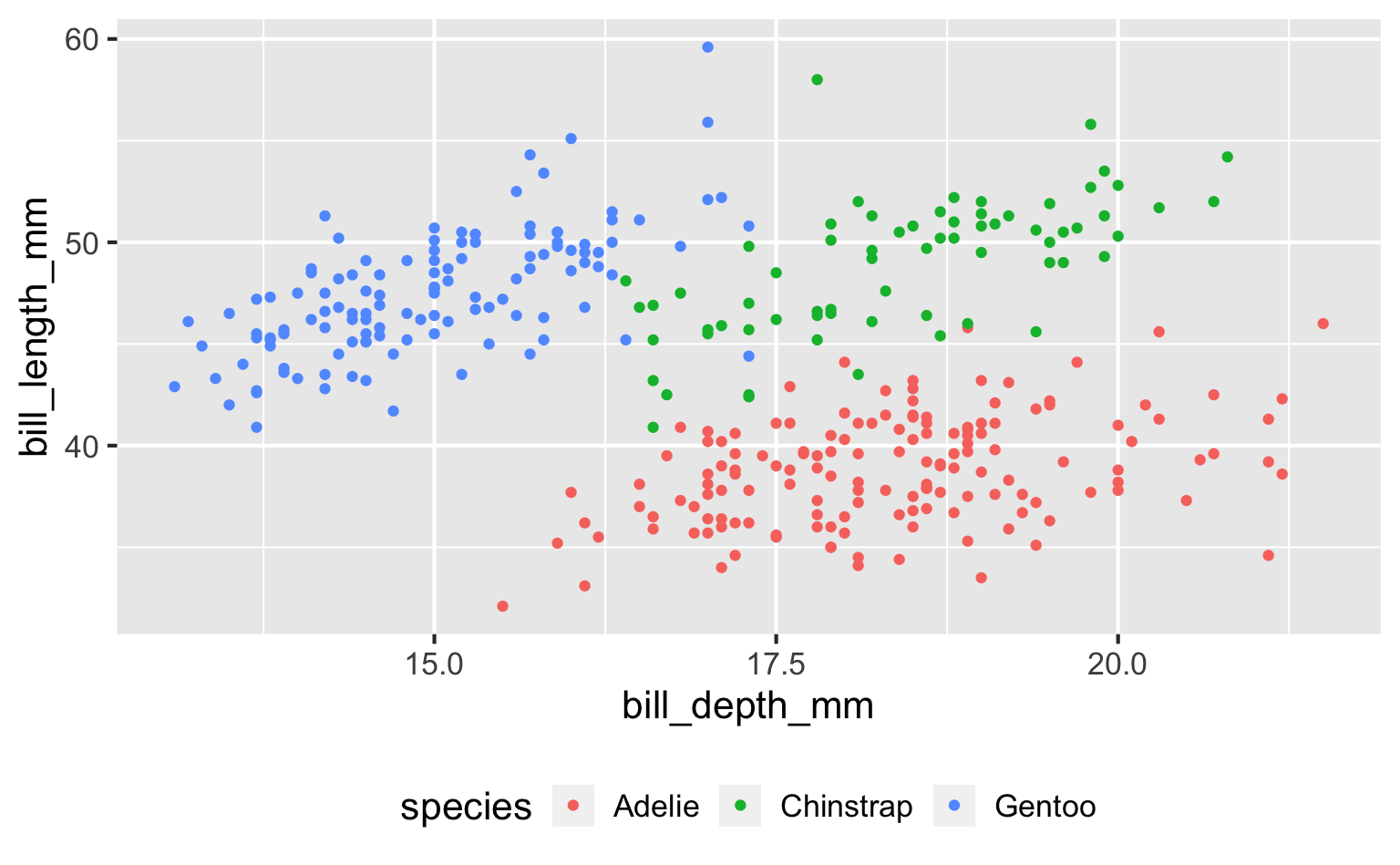

and many more throughout the course…