Rows: 10,000
Columns: 55
$ emp_title                        <chr> "global config en…
$ emp_length                       <dbl> 3, 10, 3, 1, 10, …
$ state                            <fct> NJ, HI, WI, PA, C…
$ homeownership                    <fct> MORTGAGE, RENT, R…
$ annual_income                    <dbl> 90000, 40000, 400…
$ verified_income                  <fct> Verified, Not Ver…
$ debt_to_income                   <dbl> 18.01, 5.04, 21.1…
$ annual_income_joint              <dbl> NA, NA, NA, NA, 5…
$ verification_income_joint        <fct> , , , , Verified,…
$ debt_to_income_joint             <dbl> NA, NA, NA, NA, 3…
$ delinq_2y                        <int> 0, 0, 0, 0, 0, 1,…
$ months_since_last_delinq         <int> 38, NA, 28, NA, N…
$ earliest_credit_line             <dbl> 2001, 1996, 2006,…
$ inquiries_last_12m               <int> 6, 1, 4, 0, 7, 6,…
$ total_credit_lines               <int> 28, 30, 31, 4, 22…
$ open_credit_lines                <int> 10, 14, 10, 4, 16…
$ total_credit_limit               <int> 70795, 28800, 241…
$ total_credit_utilized            <int> 38767, 4321, 1600…
$ num_collections_last_12m         <int> 0, 0, 0, 0, 0, 0,…
$ num_historical_failed_to_pay     <int> 0, 1, 0, 1, 0, 0,…
$ months_since_90d_late            <int> 38, NA, 28, NA, N…
$ current_accounts_delinq          <int> 0, 0, 0, 0, 0, 0,…
$ total_collection_amount_ever     <int> 1250, 0, 432, 0, …
$ current_installment_accounts     <int> 2, 0, 1, 1, 1, 0,…
$ accounts_opened_24m              <int> 5, 11, 13, 1, 6, …
$ months_since_last_credit_inquiry <int> 5, 8, 7, 15, 4, 5…
$ num_satisfactory_accounts        <int> 10, 14, 10, 4, 16…
$ num_accounts_120d_past_due       <int> 0, 0, 0, 0, 0, 0,…
$ num_accounts_30d_past_due        <int> 0, 0, 0, 0, 0, 0,…
$ num_active_debit_accounts        <int> 2, 3, 3, 2, 10, 1…
$ total_debit_limit                <int> 11100, 16500, 430…
$ num_total_cc_accounts            <int> 14, 24, 14, 3, 20…
$ num_open_cc_accounts             <int> 8, 14, 8, 3, 15, …
$ num_cc_carrying_balance          <int> 6, 4, 6, 2, 13, 5…
$ num_mort_accounts                <int> 1, 0, 0, 0, 0, 3,…
$ account_never_delinq_percent     <dbl> 92.9, 100.0, 93.5…
$ tax_liens                        <int> 0, 0, 0, 1, 0, 0,…
$ public_record_bankrupt           <int> 0, 1, 0, 0, 0, 0,…
$ loan_purpose                     <fct> moving, debt_cons…
$ application_type                 <fct> individual, indiv…
$ loan_amount                      <int> 28000, 5000, 2000…
$ term                             <dbl> 60, 36, 36, 36, 3…
$ interest_rate                    <dbl> 14.07, 12.61, 17.…
$ installment                      <dbl> 652.53, 167.54, 7…
$ grade                            <fct> C, C, D, A, C, A,…
$ sub_grade                        <fct> C3, C1, D1, A3, C…
$ issue_month                      <fct> Mar-2018, Feb-201…
$ loan_status                      <fct> Current, Current,…
$ initial_listing_status           <fct> whole, whole, fra…
$ disbursement_method              <fct> Cash, Cash, Cash,…
$ balance                          <dbl> 27015.86, 4651.37…
$ paid_total                       <dbl> 1999.330, 499.120…
$ paid_principal                   <dbl> 984.14, 348.63, 1…
$ paid_interest                    <dbl> 1015.19, 150.49, …
$ paid_late_fees <dbl> 0, 0, 0, 0, 0, 0,…Visualizing and summarizing categorical data
Data visualization and transformation
Data: Lending Club
- Thousands of loans made through the Lending Club, which is a platform that allows individuals to lend to other individuals

Not all loans are created equal – ease of getting a loan depends on (apparent) ability to pay back the loan
Data includes loans made, these are not loan applications
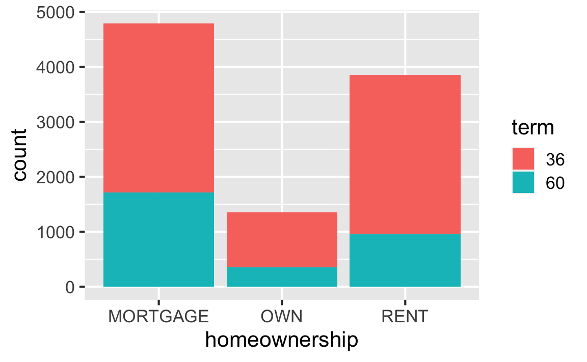
Bar plot

Segmented bar plot
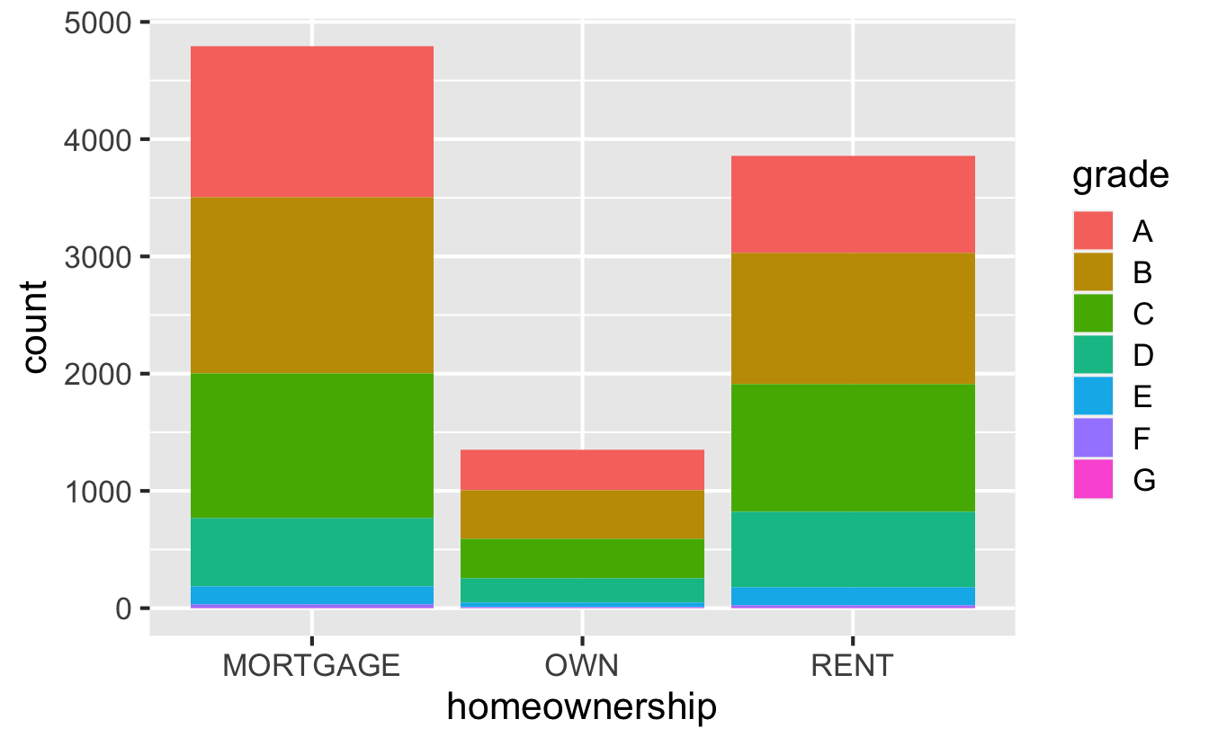
Segmented bar plot
Warning: The following aesthetics were dropped during statistical
transformation: fill
ℹ This can happen when ggplot fails to infer the correct
  grouping structure in the data.
ℹ Did you forget to specify a `group` aesthetic or to
  convert a numerical variable into a factor?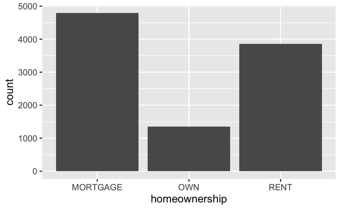
Numerical to categorical

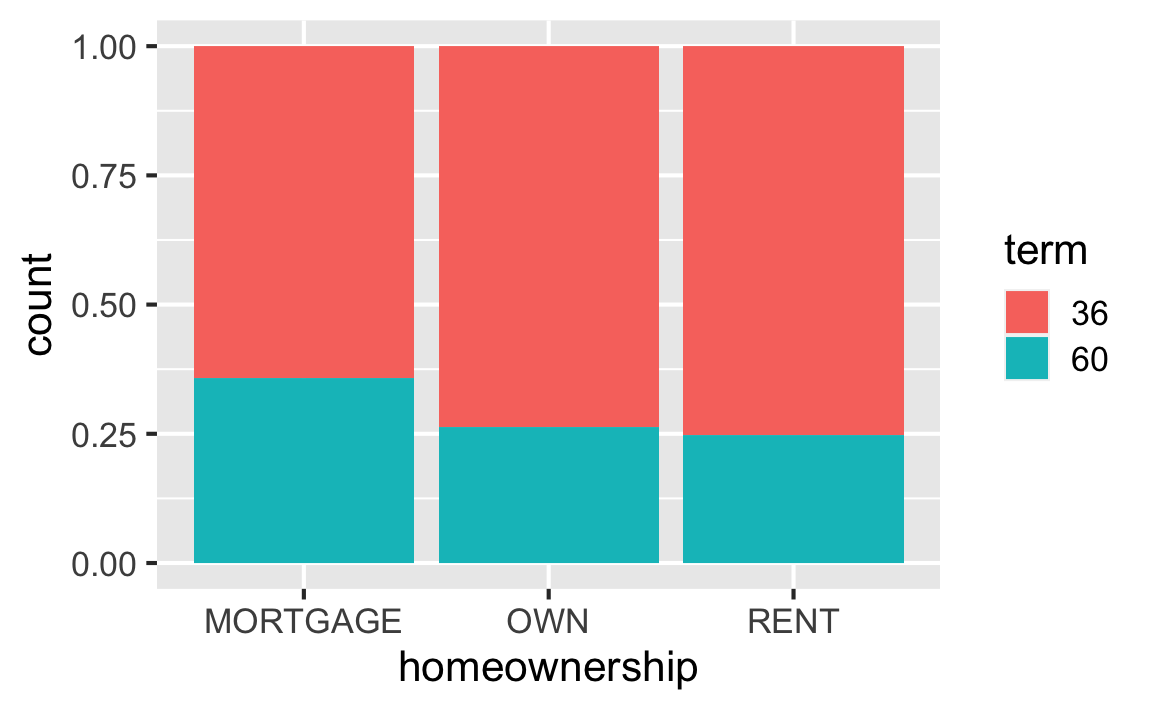
Segmented bar plot - proportions
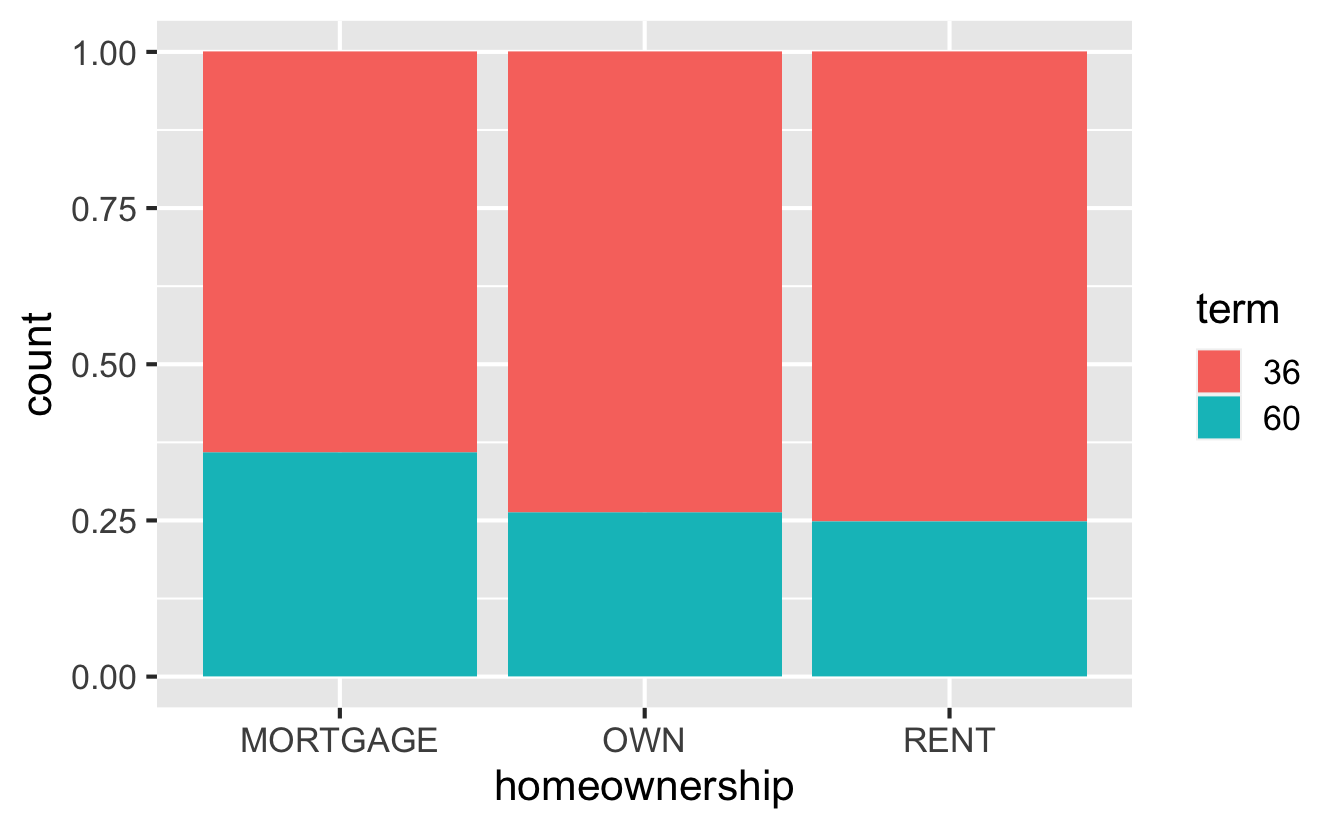
Frequencies vs. proportions
Which bar plot is a more useful representation for visualizing the relationship between homeownership and term?
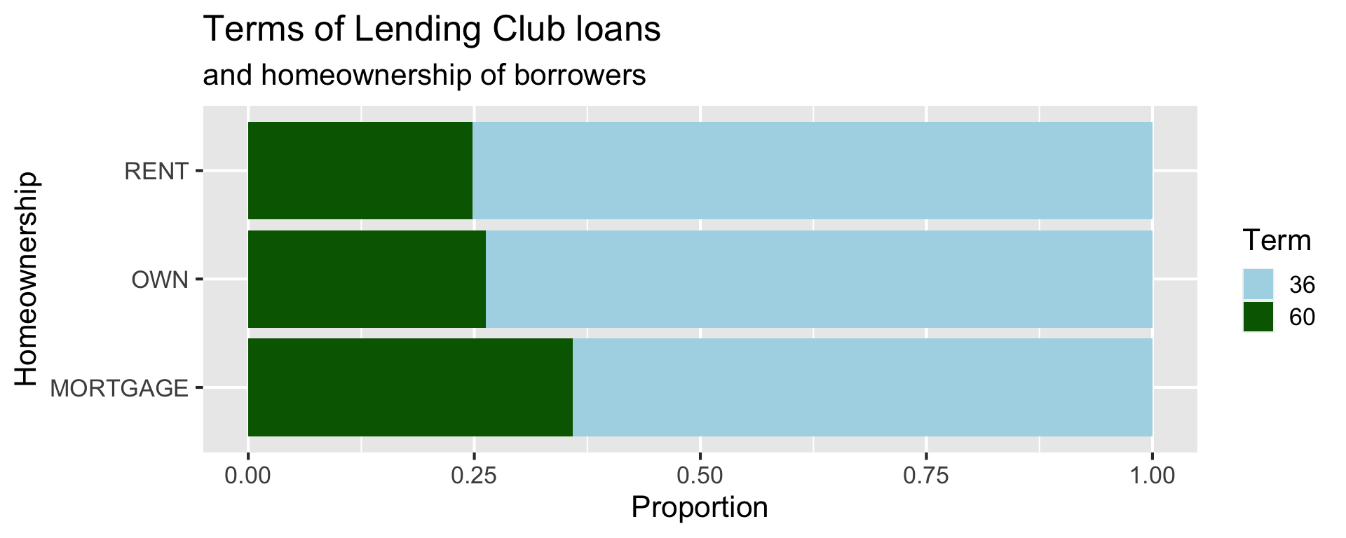
Customizing bar plots
loans |>
  mutate(term = as.factor(term)) |>
  ggplot(aes(y = homeownership, fill = term)) +
  geom_bar(position = "fill") +
  labs(
    x = "Proportion", y = "Homeownership", fill = "Term",
    title = "Terms of Lending Club loans",
    subtitle = "and homeownership of borrowers"
  ) +
  scale_fill_manual(values = c("lightblue", "darkgreen"))