Visualizing and summarizing numerical data
Data visualization and transformation
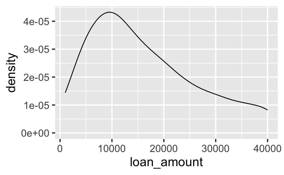
Loan amount

Shape
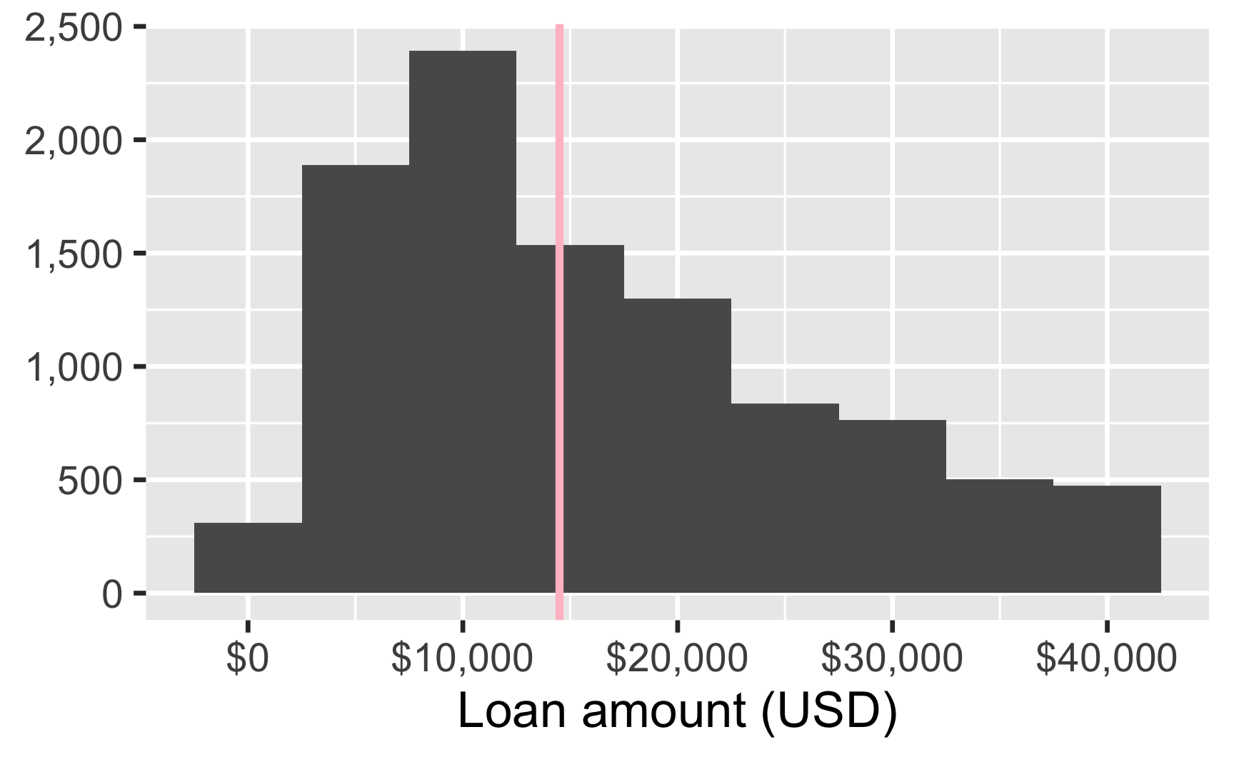
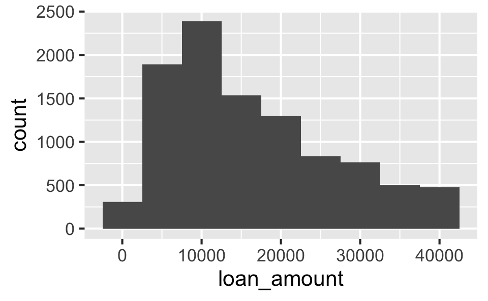
The distribution of loan amounts in this sample is unimodal and right-skewed distribution.
Center
Median loan amount in this sample is $14,500.
Spread
In this sample, the middle 50% of the loan amounts are between $8,000 and $24,000.
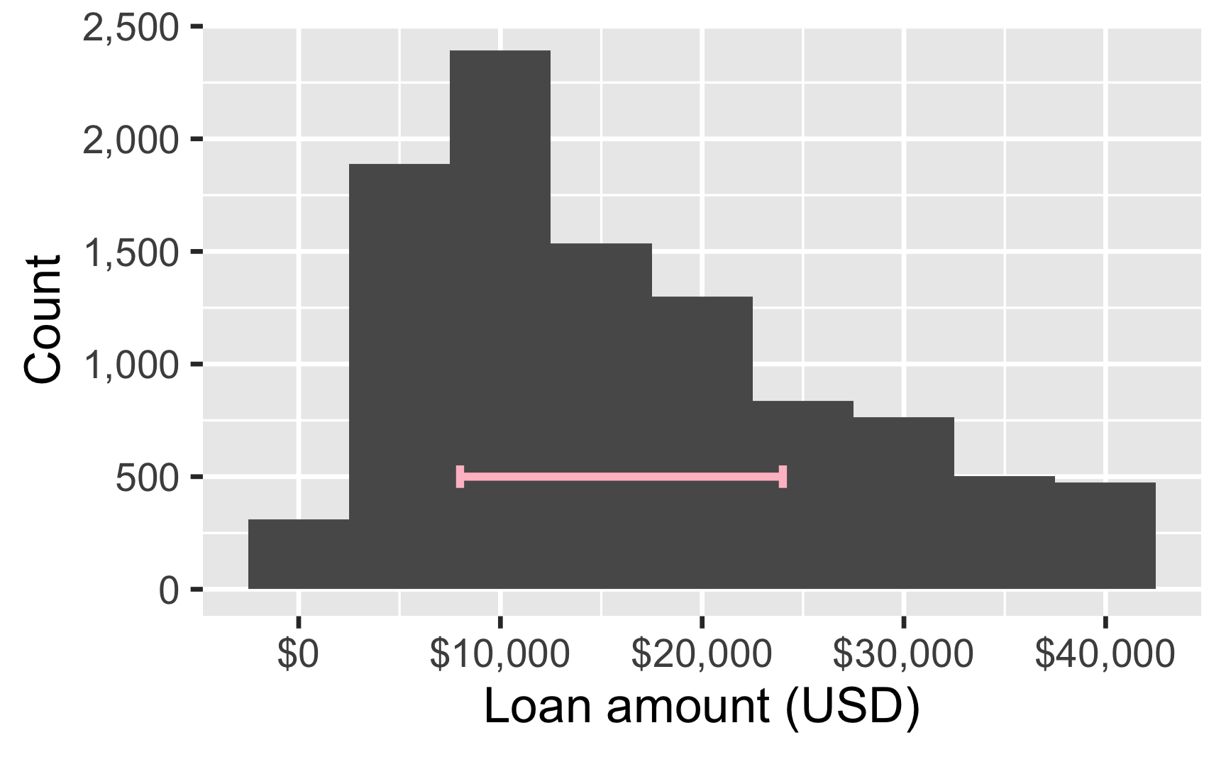
Outliers
There are no clear outliers in the loan amounts in this sample.
Histogram
- Helpful for identifying shape (modality and skewness)
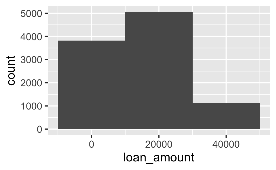
- Requires a careful selection of binwidth
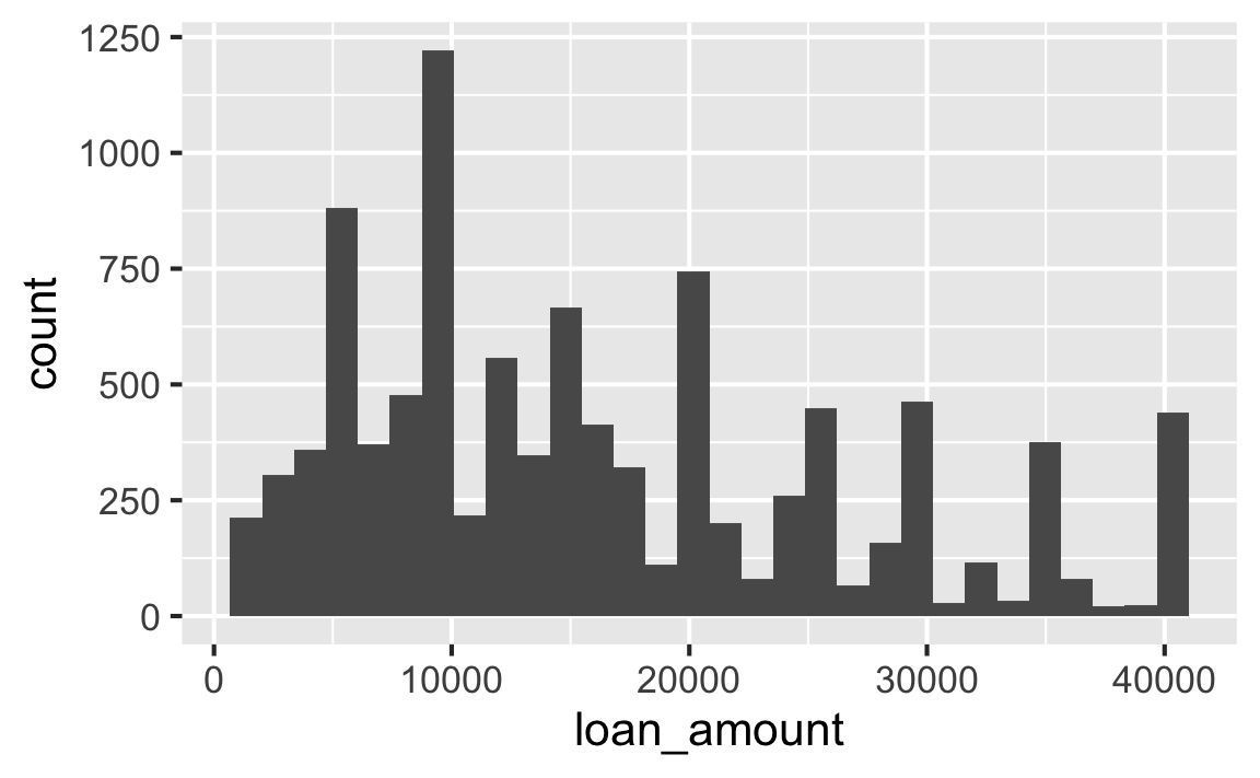
Histograms and binwidth
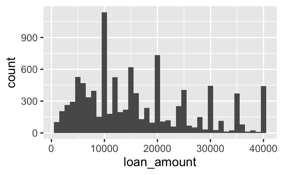
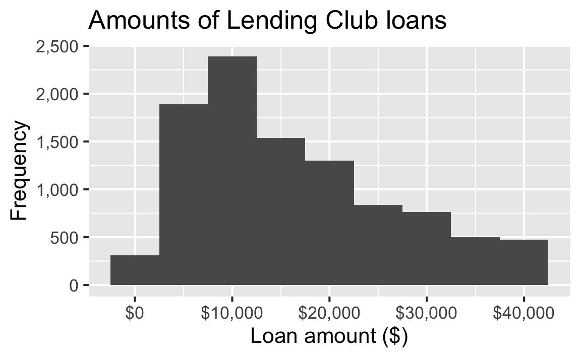
Histogram customization
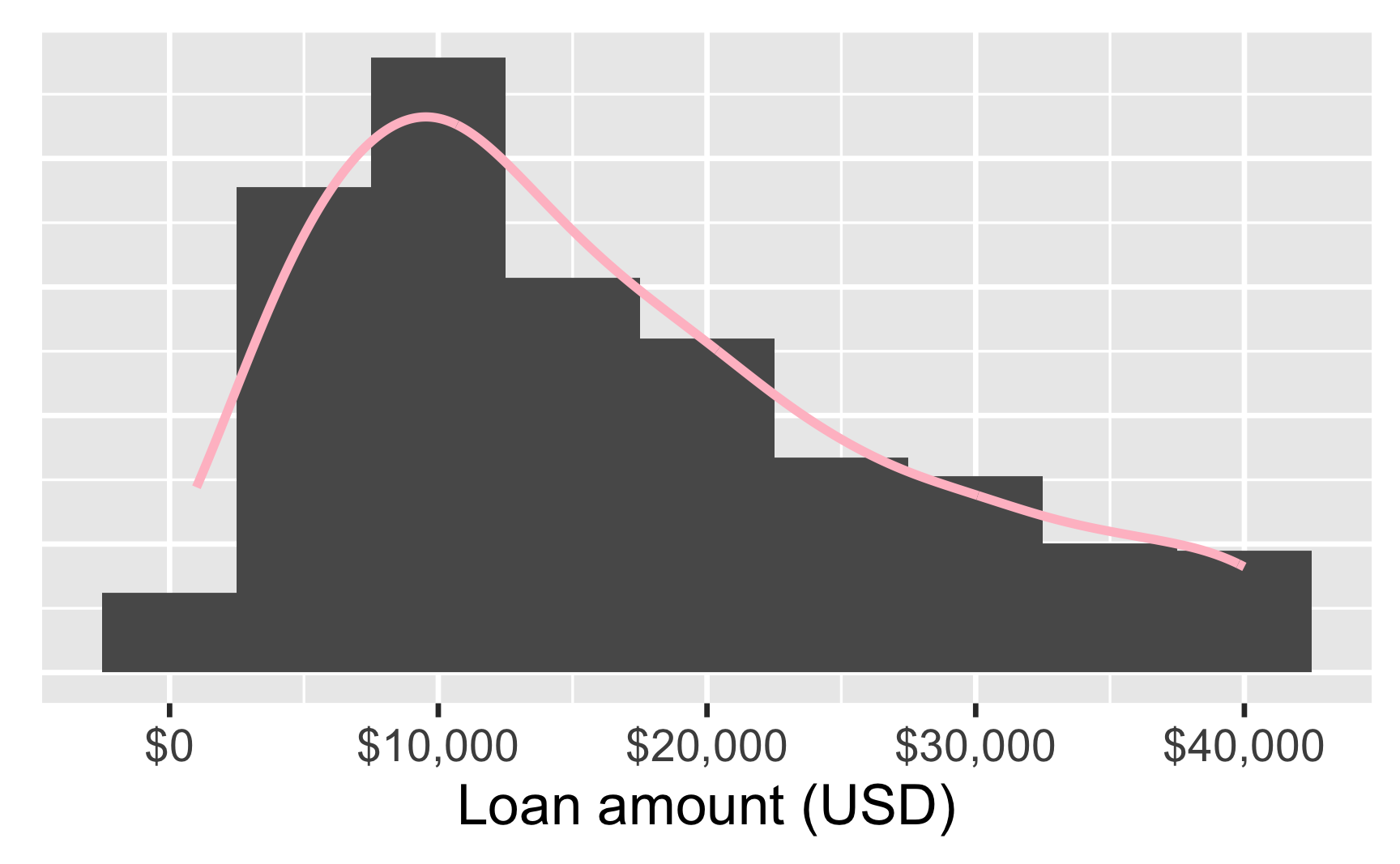
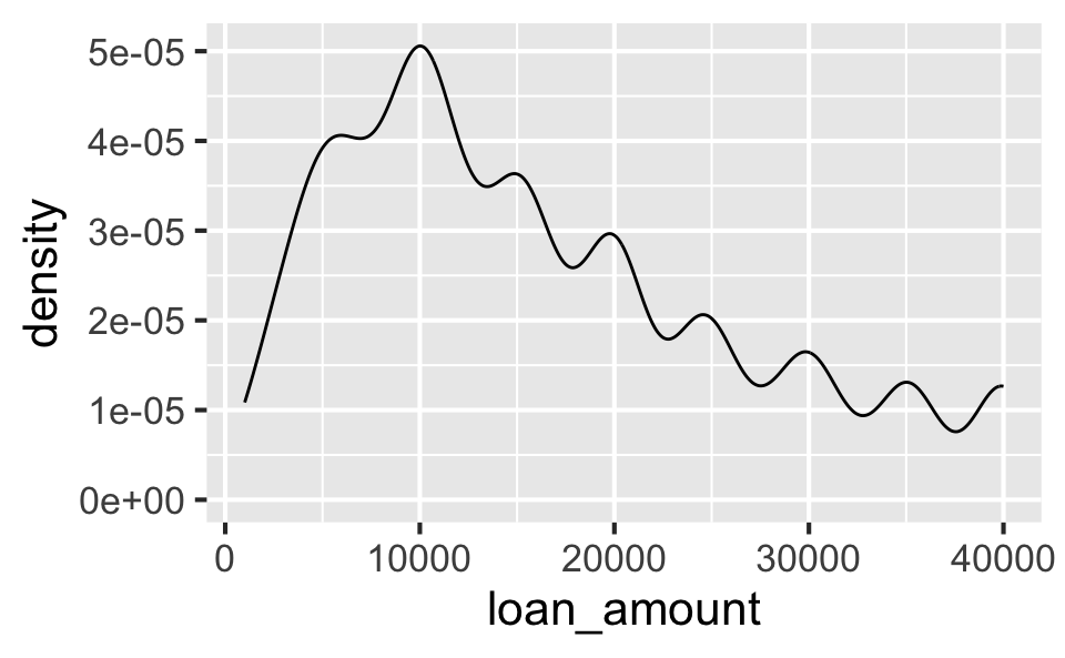
Density plot
- Helpful for identifying shape (modality and skewness)
- Smoothness can be
adjusted
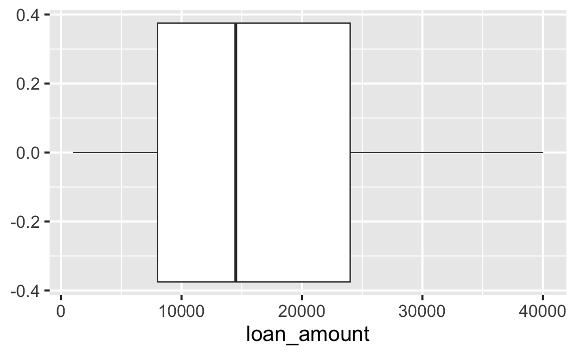
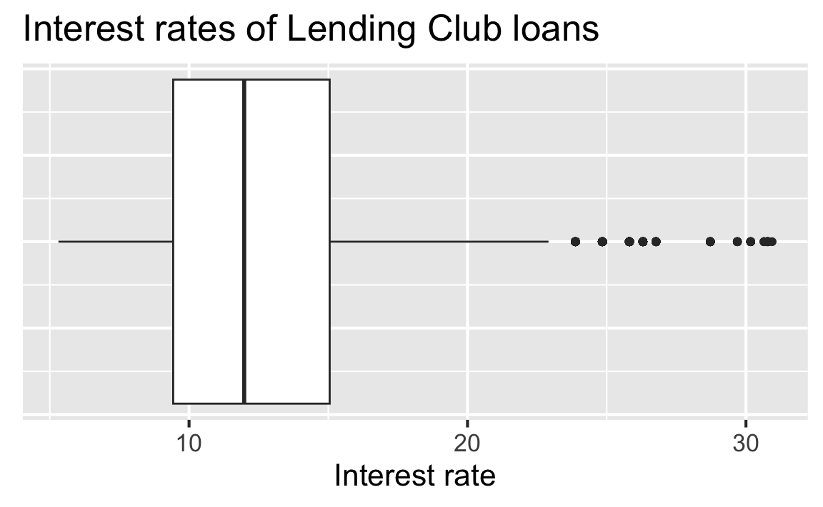
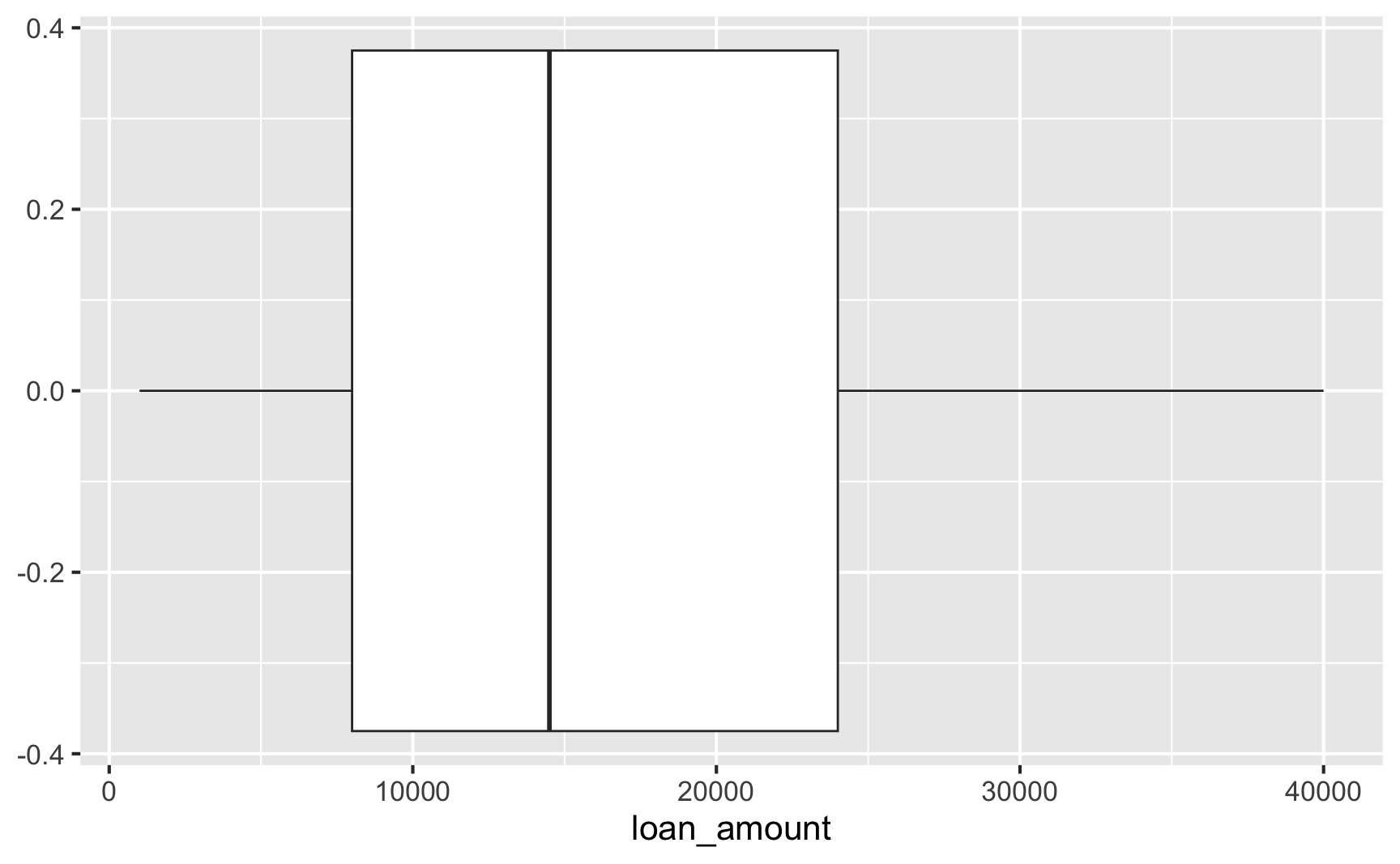
Box plot
- Helpful for identifying min, max, 25th percentile, median (50th percentile), 75th percentile
- Helpful for identifying shape (skewness, but not modality)
- Makes outliers very clear (according to a strict definition of an outlier)