Visualizing and summarizing relationships

Data visualization and transformation

Data Science with R

Setup

Packages

library(tidyverse) # for data wrangling and visualization
library(openintro) # for data
library(scales)    # for pretty axis labels

Data: Houses in Duke Forest

glimpse(duke_forest)

Rows: 98
Columns: 13
$ address    <chr> "1 Learned Pl, Durham, NC 27705", "1616…
$ price      <dbl> 1520000, 1030000, 420000, 680000, 42850…
$ bed        <dbl> 3, 5, 2, 4, 4, 3, 5, 4, 4, 3, 4, 4, 3, …
$ bath       <dbl> 4.0, 4.0, 3.0, 3.0, 3.0, 3.0, 5.0, 3.0,…
$ area       <dbl> 6040, 4475, 1745, 2091, 1772, 1950, 390…
$ type       <chr> "Single Family", "Single Family", "Sing…
$ year_built <dbl> 1972, 1969, 1959, 1961, 2020, 2014, 196…
$ heating    <chr> "Other, Gas", "Forced air, Gas", "Force…
$ cooling    <fct> central, central, central, central, cen…
$ parking    <chr> "0 spaces", "Carport, Covered", "Garage…
$ lot        <dbl> 0.97, 1.38, 0.51, 0.84, 0.16, 0.45, 0.9…
$ hoa        <chr> NA, NA, NA, NA, NA, NA, NA, NA, NA, NA,…
$ url        <chr> "https://www.zillow.com/homedetails/1-L…

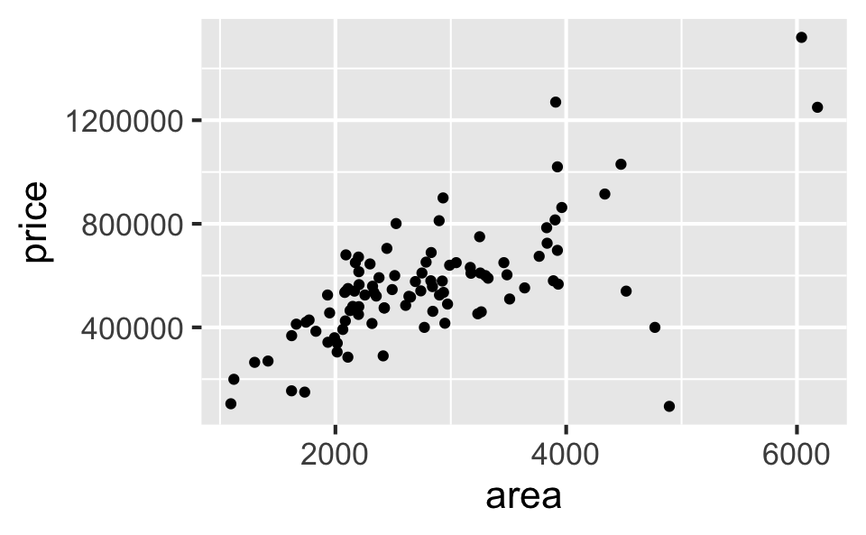
Price vs. area

Relationship between two numerical variables

Scatterplot

ggplot(duke_forest, aes(x = area, y = price)) +
  geom_point()

Correlation coefficient

duke_forest |>
  summarize(r = cor(area, price))

# A tibble: 1 × 1
      r
  <dbl>
1 0.667

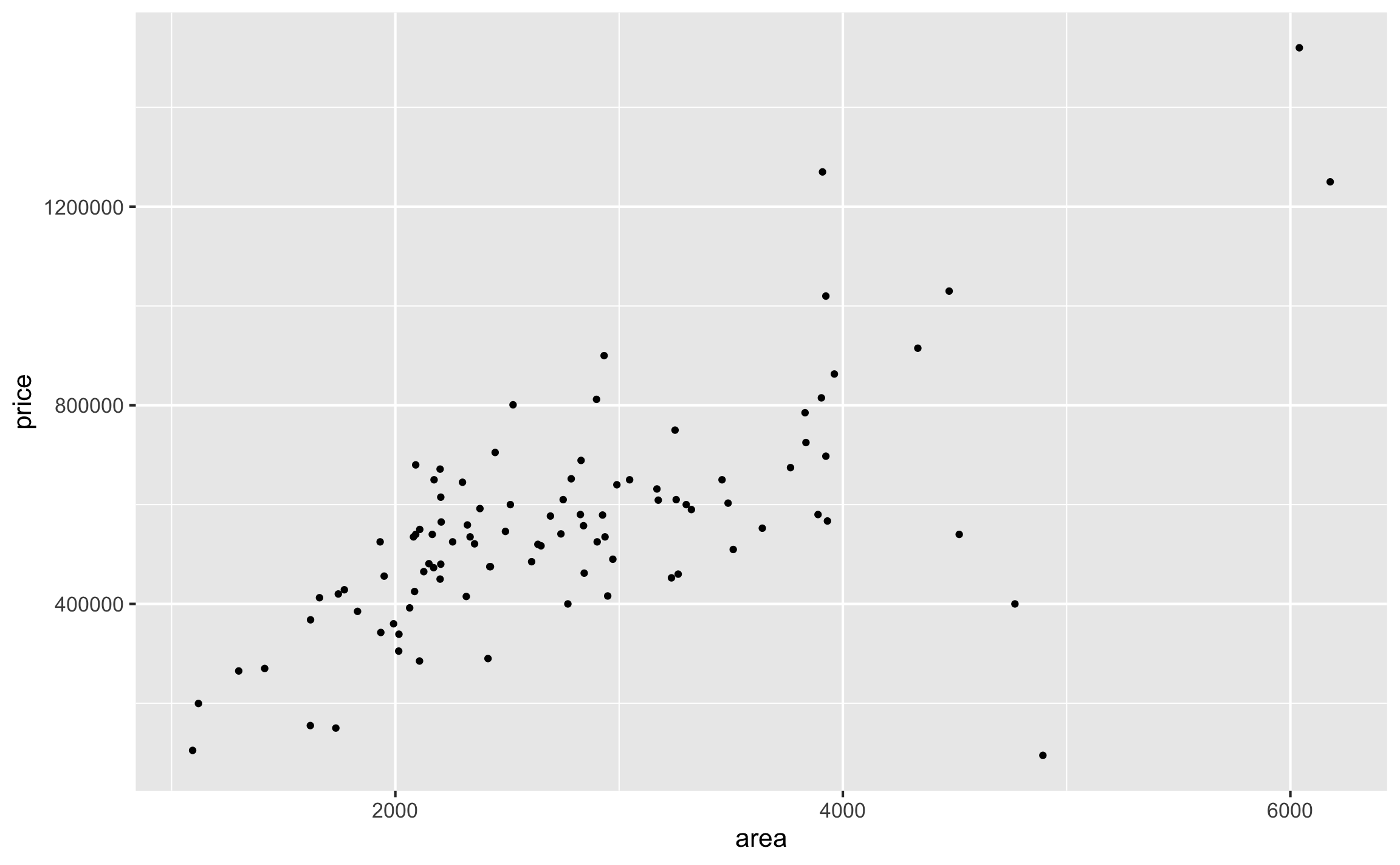
Characteristics of a relationship

between two numerical variables

Direction: Positive
Strength: Moderately strong
Form: Linear

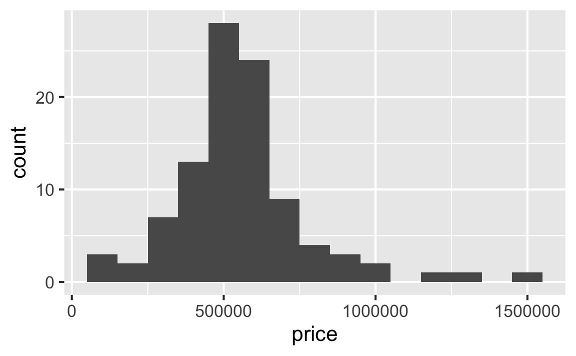
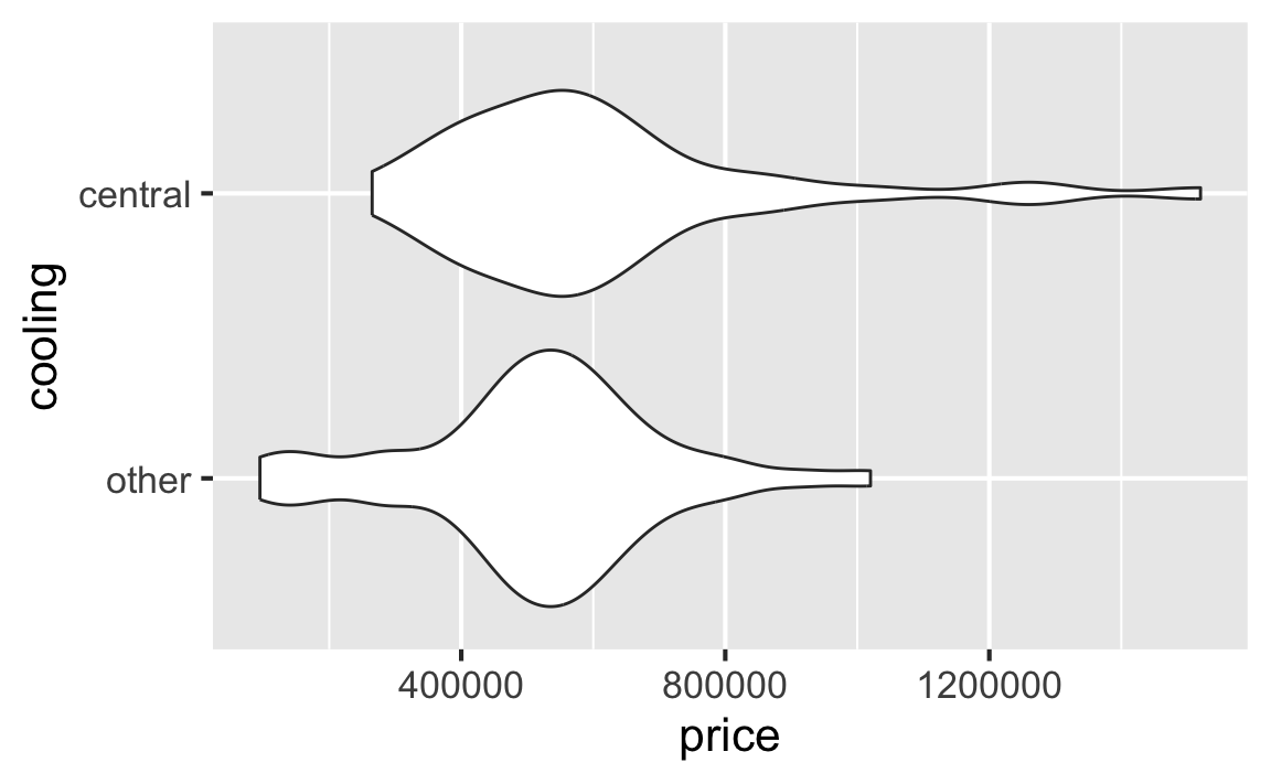
Relationship between a numerical and a categorical variable

Distribution of house prices

ggplot(duke_forest, aes(x = price)) +
  geom_histogram(binwidth = 100000)

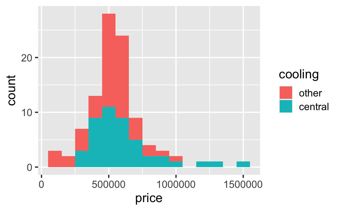
Filled histograms

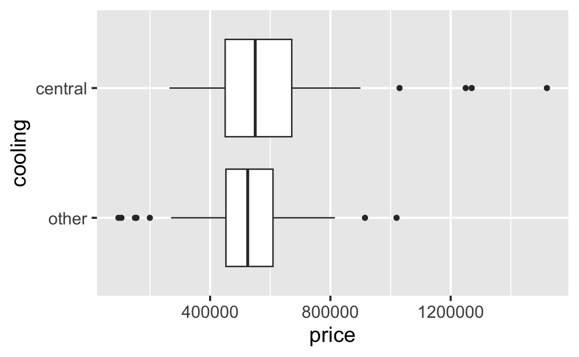
ggplot(duke_forest, aes(x = price, fill = cooling)) +
  geom_histogram(binwidth = 100000)

Side-by-side box plots

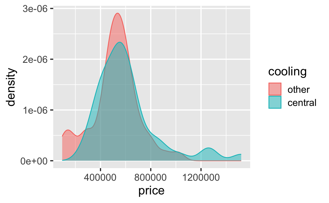
ggplot(duke_forest, aes(x = price, y = cooling)) +
  geom_boxplot()

Filled density plots

ggplot(
  duke_forest, 
  aes(x = price, color = cooling, fill = cooling)
  ) +
  geom_density(alpha = 0.5)

Violin plots

ggplot(duke_forest, aes(x = price, y = cooling)) +
  geom_violin()

Grouped summaries

duke_forest |>
  group_by(cooling) |>
  summarize(median_price = median(price))

# A tibble: 2 × 2
  cooling median_price
  <fct>          <dbl>
1 other         525000
2 central       550000

Multiple summary statistics

duke_forest |>
  group_by(cooling) |>
  summarize(
    min_price = min(price),
    median_price = median(price), 
    iqr_price = IQR(price),
    max_price = max(price)
  )

# A tibble: 2 × 5
  cooling min_price median_price iqr_price max_price
  <fct>       <dbl>        <dbl>     <dbl>     <dbl>
1 other       95000       525000    156500   1020000
2 central    265000       550000    221500   1520000

Relationship between two categorical variables

Year built

Create a new variable called year_built_cat that takes on the value "1970 or later" if the house is built in 1970 or later, and "1969 or earlier" otherwise.

duke_forest <- duke_forest |>
  mutate(
    year_built_cat = if_else(
      year_built >= 1970, 
      "1970 or later", 
      "1969 or earlier"
    )
   )

Year built

duke_forest |>
  select(contains("year_built"))

# A tibble: 98 × 2
   year_built year_built_cat 
        <dbl> <chr>          
 1       1972 1970 or later  
 2       1969 1969 or earlier
 3       1959 1969 or earlier
 4       1961 1969 or earlier
 5       2020 1970 or later  
 6       2014 1970 or later  
 7       1968 1969 or earlier
 8       1973 1970 or later  
 9       1972 1970 or later  
10       1964 1969 or earlier
# ℹ 88 more rows

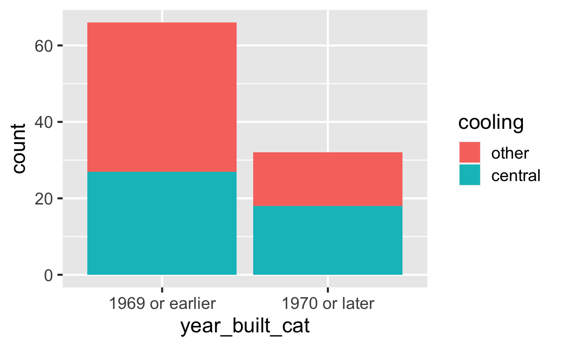
Stacked bar plot – frequencies

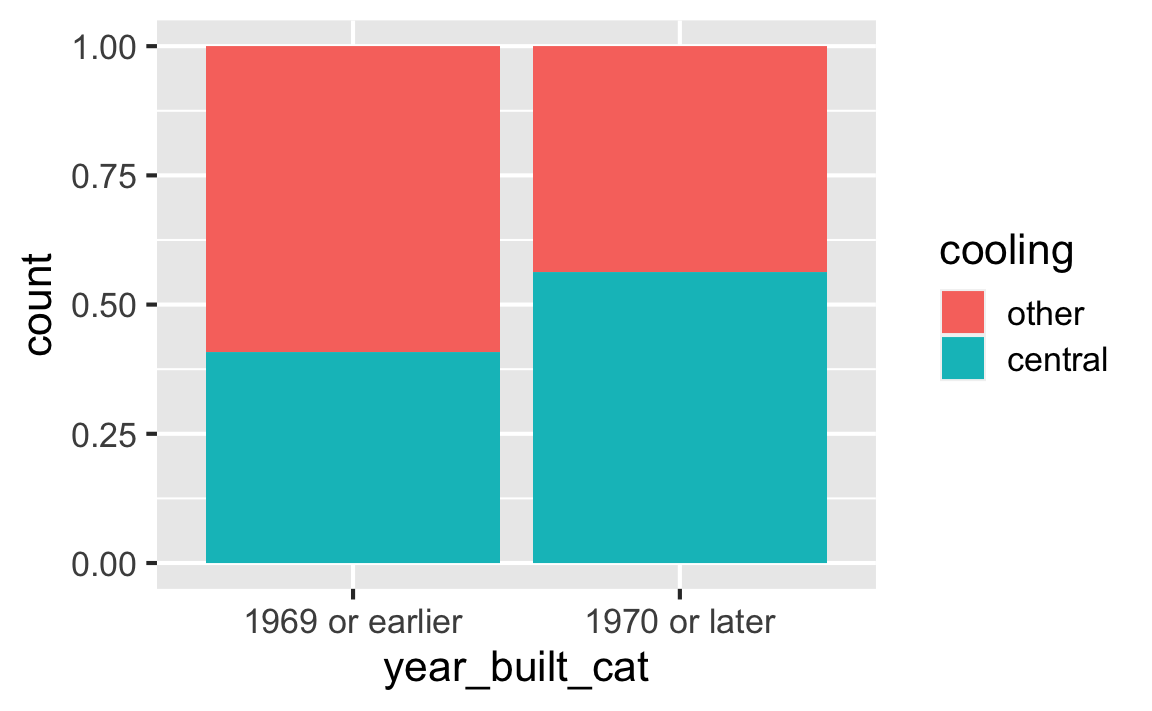
ggplot(duke_forest, aes(x = year_built_cat, fill = cooling)) +
  geom_bar()

Stacked bar plot – proportions

ggplot(duke_forest, aes(x = year_built_cat, fill = cooling)) +
  geom_bar(position = "fill")

Frequencies

duke_forest |>
  count(year_built_cat, cooling)

# A tibble: 4 × 3
  year_built_cat  cooling     n
  <chr>           <fct>   <int>
1 1969 or earlier other      39
2 1969 or earlier central    27
3 1970 or later   other      14
4 1970 or later   central    18

Proportions

duke_forest |>
  count(year_built_cat, cooling) |>
  group_by(year_built_cat) |>
  mutate(prop = n / sum(n))

# A tibble: 4 × 4
# Groups:   year_built_cat [2]
  year_built_cat  cooling     n  prop
  <chr>           <fct>   <int> <dbl>
1 1969 or earlier other      39 0.591
2 1969 or earlier central    27 0.409
3 1970 or later   other      14 0.438
4 1970 or later   central    18 0.562

Relationships between many variables

Price vs. area and cooling - 1

ggplot(
  duke_forest, 
  aes(
    x = area, y = price, 
    color = cooling, shape = cooling
    )
  ) +
  geom_point()

Price vs. area and cooling - 2

ggplot(
  duke_forest, 
  aes(
    x = area, y = price, 
    color = cooling, shape = cooling
    )
  ) +
  geom_point(alpha = 0.7, size = 4)

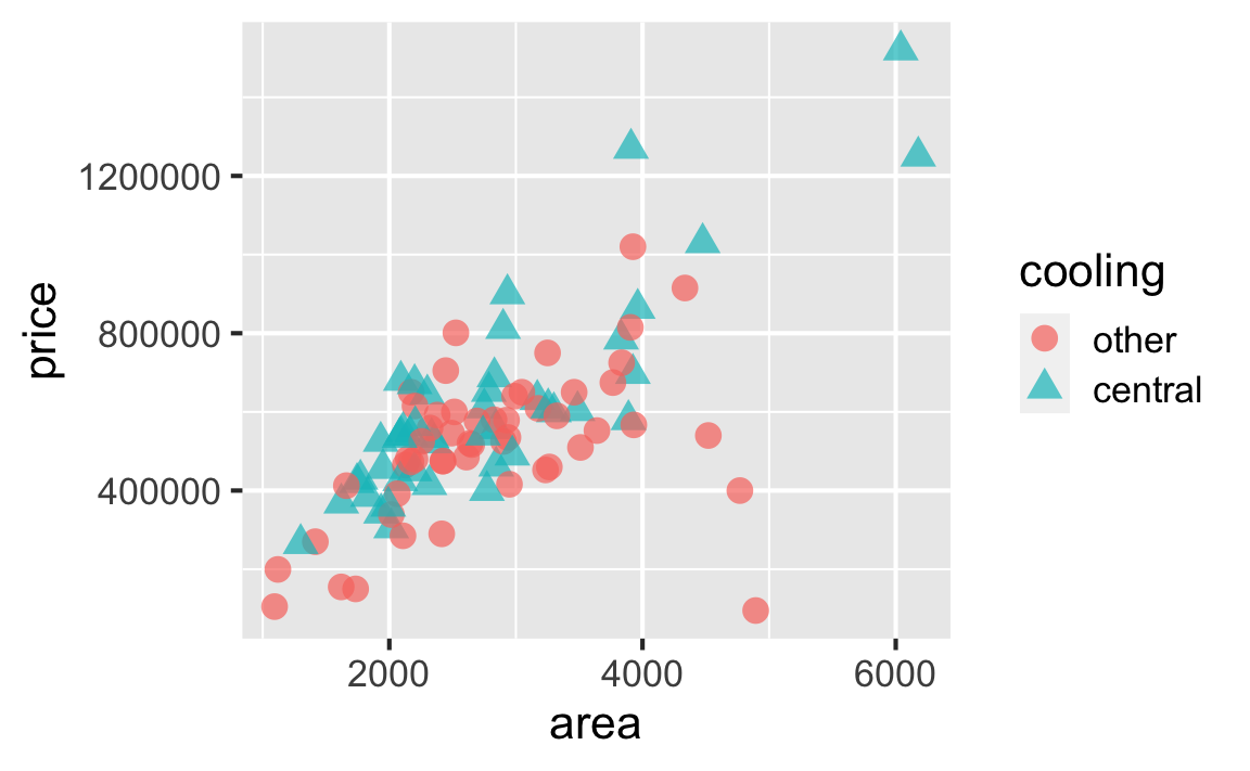
Price vs. area and cooling - 3

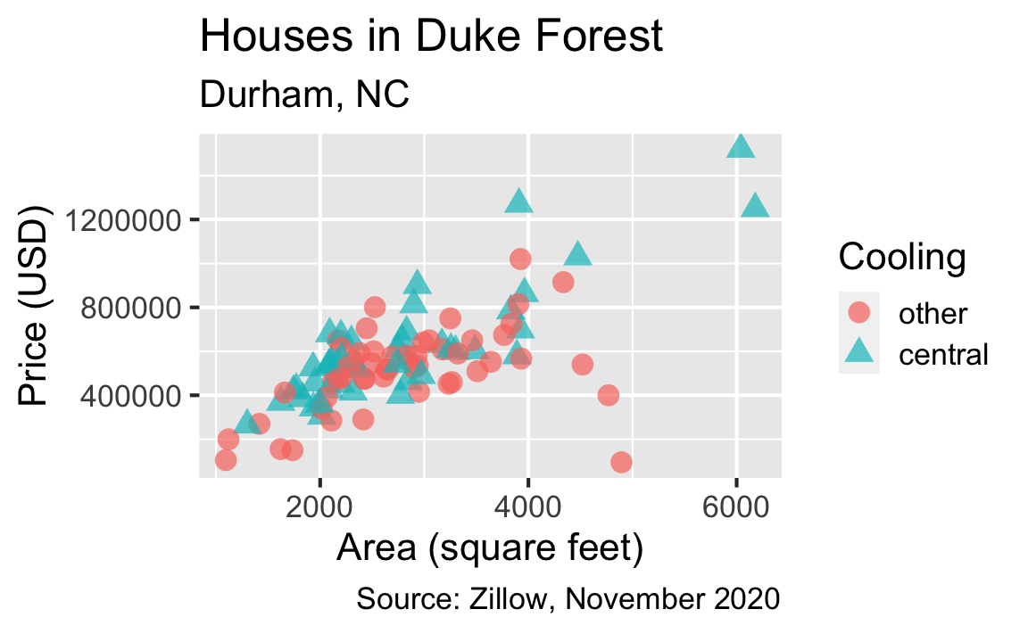
ggplot(
  duke_forest, 
  aes(
    x = area, y = price, 
    color = cooling, shape = cooling
    )
  ) +
  geom_point(alpha = 0.7, size = 4) +
  labs(
    title = "Houses in Duke Forest",
    subtitle = "Durham, NC",
    color = "Cooling", shape = "Cooling",
    x = "Area (square feet)",
    y = "Price (USD)",
    caption = "Source: Zillow, November 2020"
  )

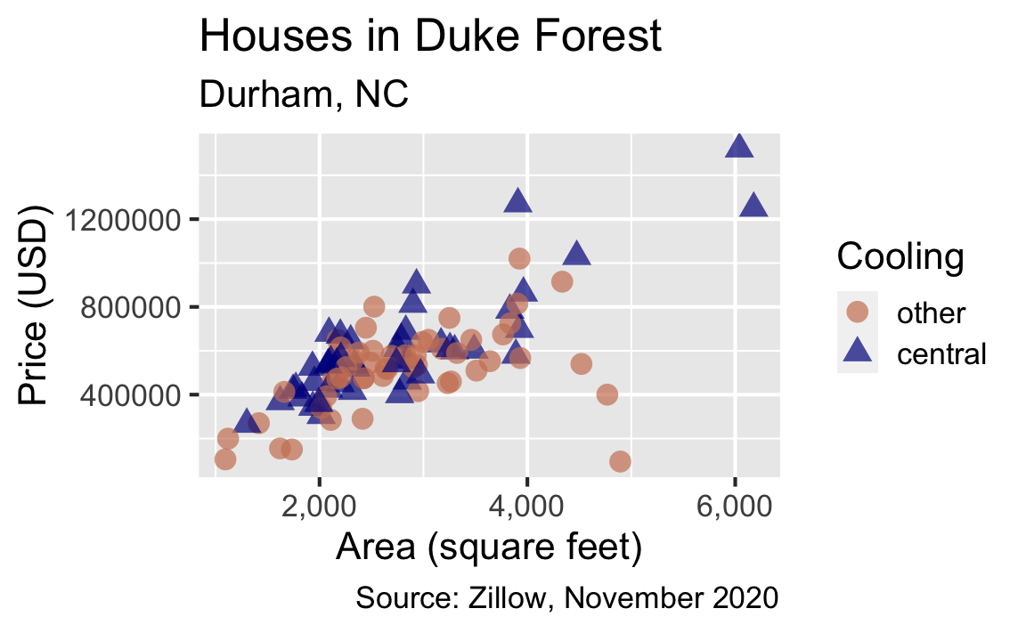
Price vs. area and cooling - 4

ggplot(
  duke_forest, 
  aes(
    x = area, y = price, 
    color = cooling, shape = cooling
    )
  ) +
  geom_point(alpha = 0.7, size = 4) +
  scale_color_manual(
    values = c("central" = "darkblue", "other" = "lightsalmon3")
    ) +
  labs(
    title = "Houses in Duke Forest",
    subtitle = "Durham, NC",
    color = "Cooling", shape = "Cooling",
    x = "Area (square feet)",
    y = "Price (USD)",
    caption = "Source: Zillow, November 2020"
  )

Price vs. area and cooling - 5

ggplot(
  duke_forest, 
  aes(
    x = area, y = price, 
    color = cooling, shape = cooling
    )
  ) +
  geom_point(alpha = 0.7, size = 4) +
  scale_x_continuous(labels = label_number(big.mark = ",")) +
  scale_color_manual(
    values = c("central" = "darkblue", "other" = "lightsalmon3")
    ) +
  labs(
    title = "Houses in Duke Forest",
    subtitle = "Durham, NC",
    color = "Cooling", shape = "Cooling",
    x = "Area (square feet)",
    y = "Price (USD)",
    caption = "Source: Zillow, November 2020"
  )

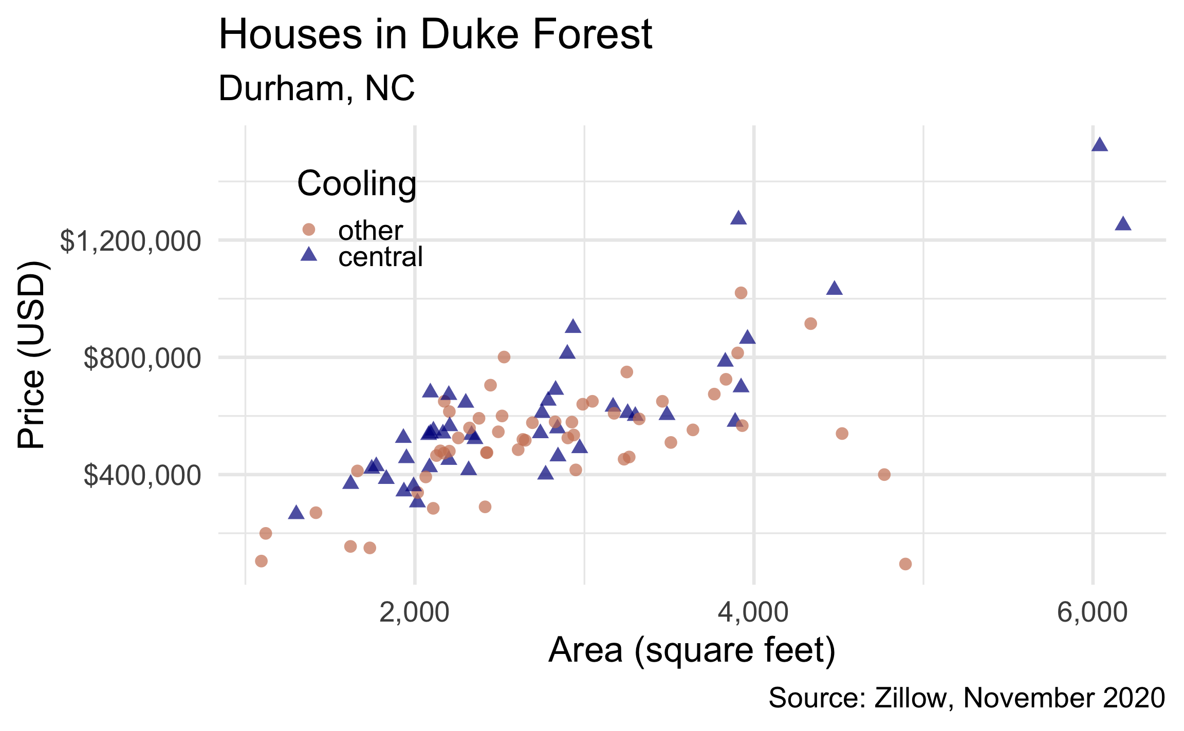
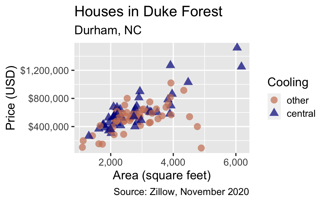
Price vs. area and cooling - 6

ggplot(
  duke_forest, 
  aes(
    x = area, y = price, 
    color = cooling, shape = cooling
    )
  ) +
  geom_point(alpha = 0.7, size = 4) +
  scale_x_continuous(labels = label_number(big.mark = ",")) +
  scale_y_continuous(labels = label_dollar()) +
  scale_color_manual(
    values = c("central" = "darkblue", "other" = "lightsalmon3")
    ) +
  labs(
    title = "Houses in Duke Forest",
    subtitle = "Durham, NC",
    color = "Cooling", shape = "Cooling",
    x = "Area (square feet)",
    y = "Price (USD)",
    caption = "Source: Zillow, November 2020"
  )

Price vs. area and cooling - 7

duke_forest |>
  group_by(cooling) |>
  summarize(r = cor(price, area))

# A tibble: 2 × 2
  cooling     r
  <fct>   <dbl>
1 other   0.459
2 central 0.854

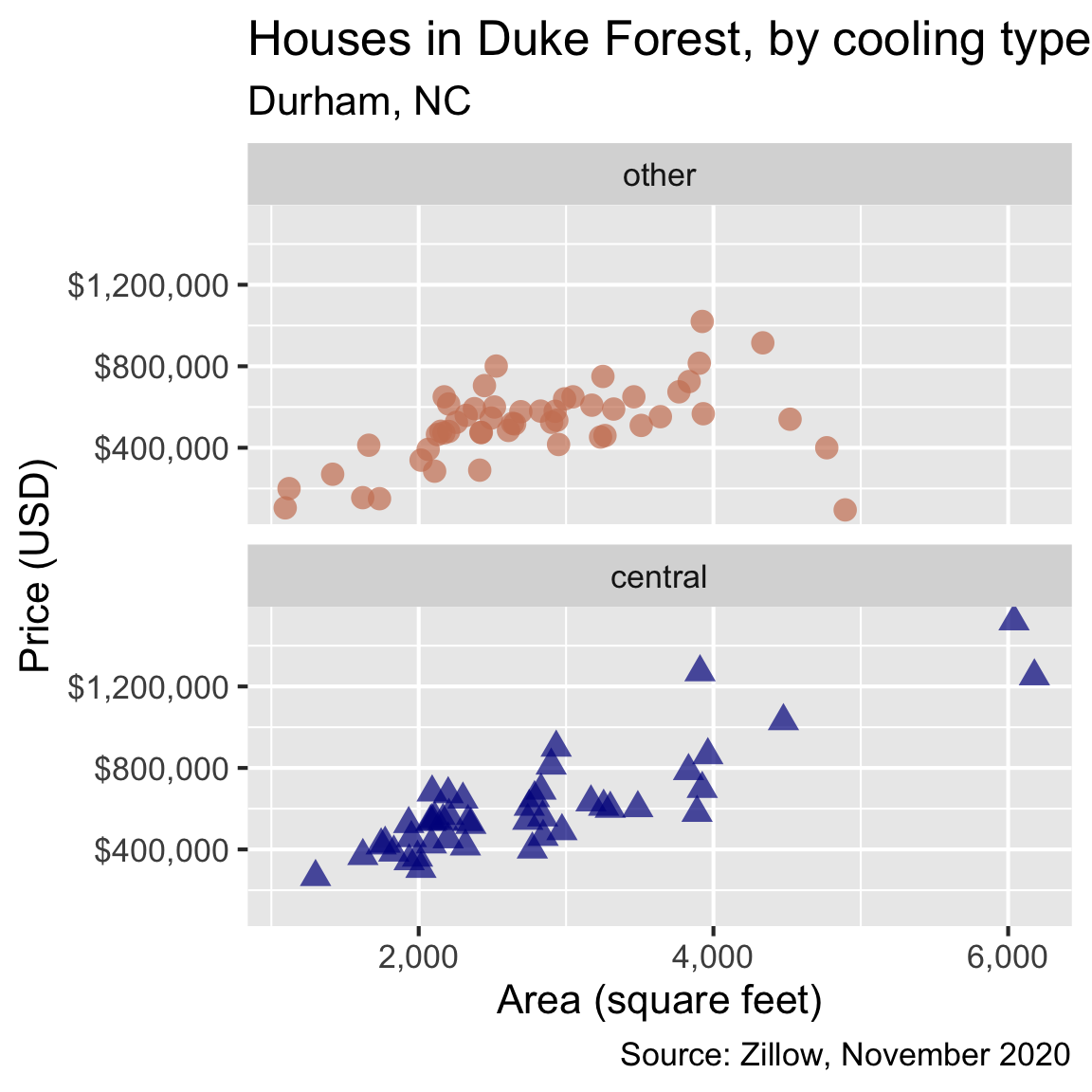
Price vs. area and cooling - 8

ggplot(
  duke_forest, 
  aes(
    x = area, y = price, 
    color = cooling, shape = cooling
    )
  ) +
  geom_point(alpha = 0.7, size = 4) +
  scale_x_continuous(labels = label_number(big.mark = ",")) +
  scale_y_continuous(labels = label_dollar()) +
  scale_color_manual(
    values = c("central" = "darkblue", "other" = "lightsalmon3")
    ) +
  labs(
    title = "Houses in Duke Forest",
    subtitle = "Durham, NC",
    color = "Cooling", shape = "Cooling",
    x = "Area (square feet)",
    y = "Price (USD)",
    caption = "Source: Zillow, November 2020"
  ) +
  facet_wrap(~cooling, ncol = 1)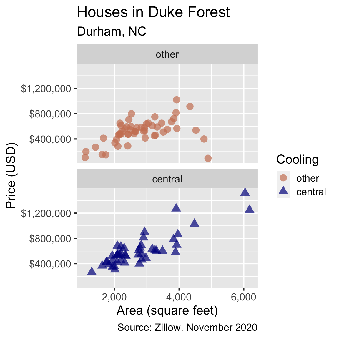

Price vs. area and cooling - 9

ggplot(
  duke_forest, 
  aes(
    x = area, y = price, 
    color = cooling, shape = cooling
    )
  ) +
  geom_point(alpha = 0.7, size = 4, show.legend = FALSE) +
  scale_x_continuous(labels = label_number(big.mark = ",")) +
  scale_y_continuous(labels = label_dollar()) +
  scale_color_manual(
    values = c("central" = "darkblue", "other" = "lightsalmon3")
    ) +
  labs(
    title = "Houses in Duke Forest, by cooling type",
    subtitle = "Durham, NC",
    color = "Cooling", shape = "Cooling",
    x = "Area (square feet)",
    y = "Price (USD)",
    caption = "Source: Zillow, November 2020"
  ) +
  facet_wrap(~cooling, ncol = 1)

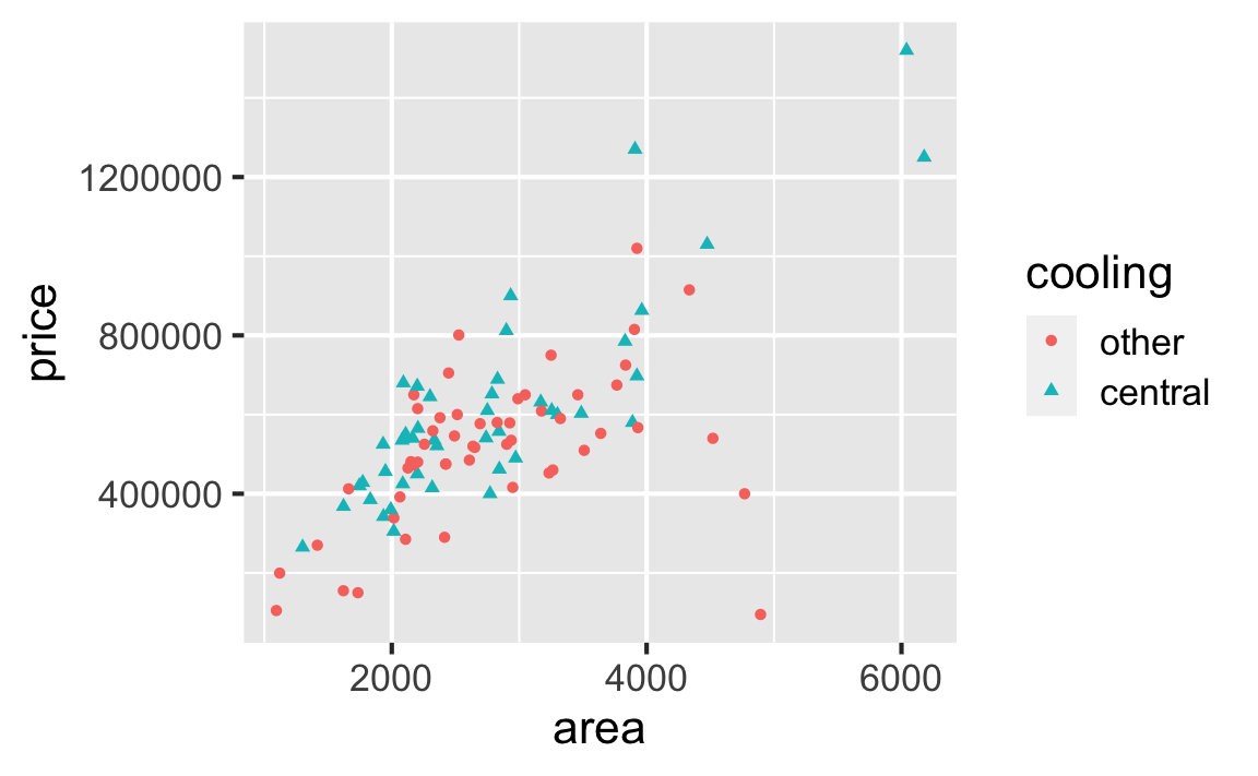
Price vs. area and cooling

The relationship between area and price of homes in Duke Forest is positive and relatively strong, regardless of cooling type.
The relationship appears to be stronger, with a larger correlation coefficient (0.854 vs. 0.459), for homes cooled with central air.
However the large difference in correlation coefficients for these two groups might be due to the three potential outliers in the other group with high areas and low price.