Modeling loan interest rates (Complete)

Introduction

Goal

Practice modeling with multiple predictors using the data on loan interest rates.

Packages

The dataset is about loans from the peer-to-peer lender, Lending Club, from the openintro package. We will use tidyverse and tidymodels for data exploration and modeling, respectively.

library(tidyverse)
library(tidymodels)
library(openintro)

Data prep

Before we use the dataset, we’ll make a few transformations to it.

Review the code below with your neighbor and write a summary of the data transformation pipeline.

Add response here.

loans <- loans_full_schema |>
  mutate(
    credit_util = total_credit_utilized / total_credit_limit,
    bankruptcy = as.factor(if_else(public_record_bankrupt == 0, 0, 1)),
    verified_income = droplevels(verified_income),
    homeownership = str_to_title(homeownership),
    homeownership = fct_relevel(homeownership, "Rent", "Mortgage", "Own")
  ) |>
  rename(credit_checks = inquiries_last_12m) |>
  select(
    interest_rate, loan_amount, verified_income, 
    debt_to_income, credit_util, bankruptcy, term, 
    credit_checks, issue_month, homeownership
  )

Here is a glimpse at the data:

glimpse(loans)

Rows: 10,000
Columns: 10
$ interest_rate   <dbl> 14.07, 12.61, 17.09, 6.72, 14.07, 6.72, 13.59, 11.99, …
$ loan_amount     <int> 28000, 5000, 2000, 21600, 23000, 5000, 24000, 20000, 2…
$ verified_income <fct> Verified, Not Verified, Source Verified, Not Verified,…
$ debt_to_income  <dbl> 18.01, 5.04, 21.15, 10.16, 57.96, 6.46, 23.66, 16.19, …
$ credit_util     <dbl> 0.54759517, 0.15003472, 0.66134832, 0.19673228, 0.7549…
$ bankruptcy      <fct> 0, 1, 0, 0, 0, 0, 0, 0, 0, 0, 1, 0, 0, 0, 1, 0, 0, 0, …
$ term            <dbl> 60, 36, 36, 36, 36, 36, 60, 60, 36, 36, 60, 60, 36, 60…
$ credit_checks   <int> 6, 1, 4, 0, 7, 6, 1, 1, 3, 0, 4, 4, 8, 6, 0, 0, 4, 6, …
$ issue_month     <fct> Mar-2018, Feb-2018, Feb-2018, Jan-2018, Mar-2018, Jan-…
$ homeownership   <fct> Mortgage, Rent, Rent, Rent, Rent, Own, Mortgage, Mortg…

Analysis

Get to know the data

What is a typical interest rate in this dataset? What are some attributes of a typical loan and a typical borrower. Give yourself no more than 5 minutes for this exploration and share 1-2 findings.

ggplot(loans, aes(x = interest_rate)) +
  geom_histogram(binwidth = 1)
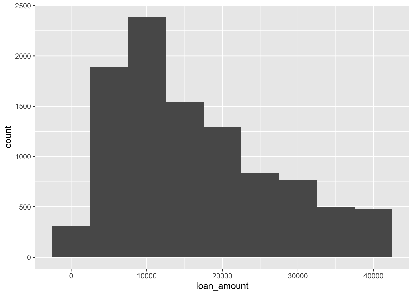
ggplot(loans, aes(x = loan_amount)) +
  geom_histogram(binwidth = 5000)
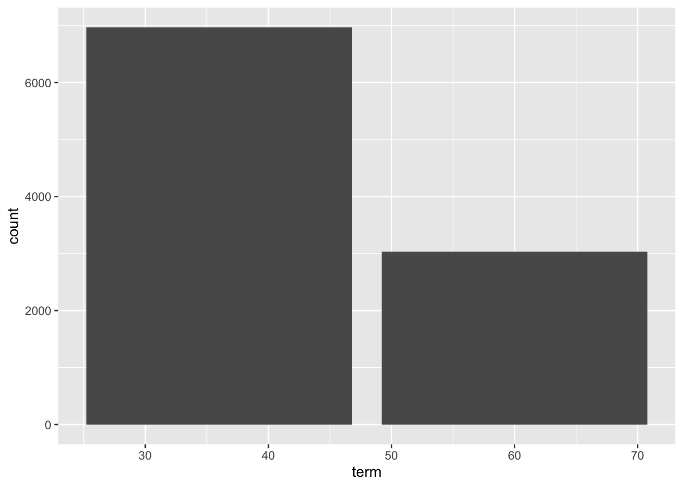
ggplot(loans, aes(x = term)) +
  geom_bar()
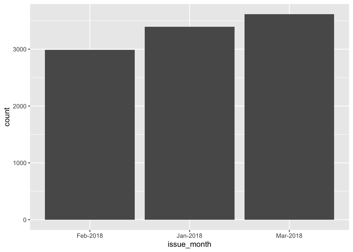
ggplot(loans, aes(x = issue_month)) +
  geom_bar()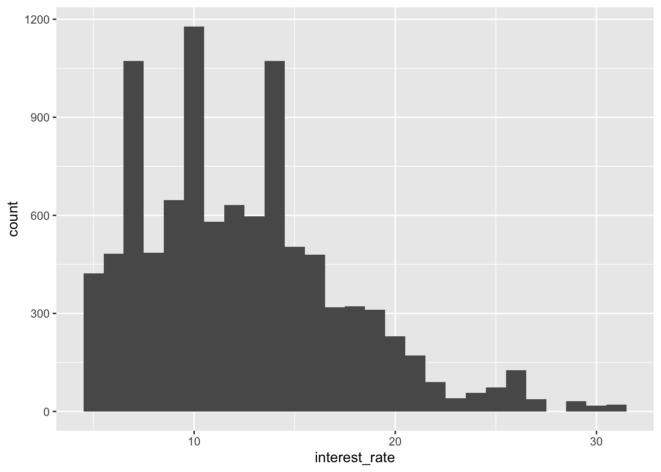

ggplot(loans, aes(x = credit_util)) +
  geom_histogram(binwidth = 0.1)
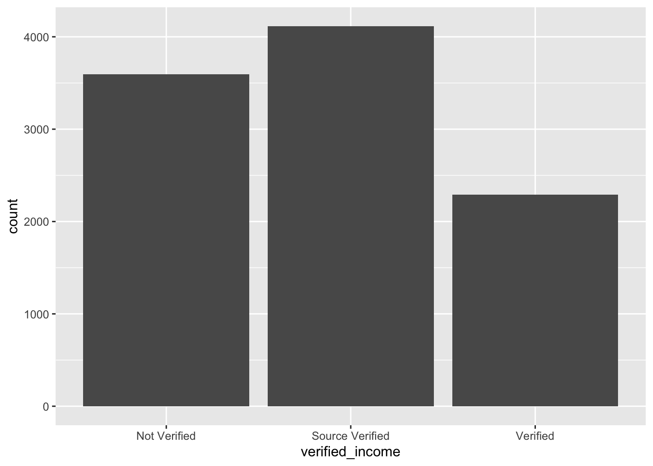
ggplot(loans, aes(x = verified_income)) +
  geom_bar()
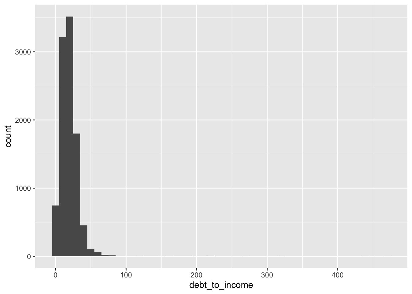
ggplot(loans, aes(x = debt_to_income)) +
  geom_histogram(binwidth = 10)
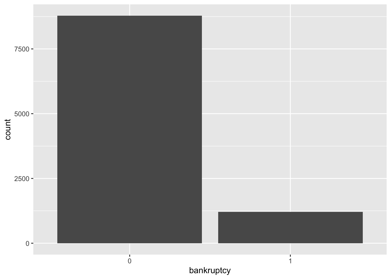
ggplot(loans, aes(x = bankruptcy)) +
  geom_bar()
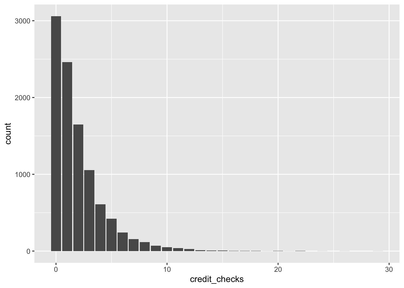
ggplot(loans, aes(x = credit_checks)) +
  geom_bar()
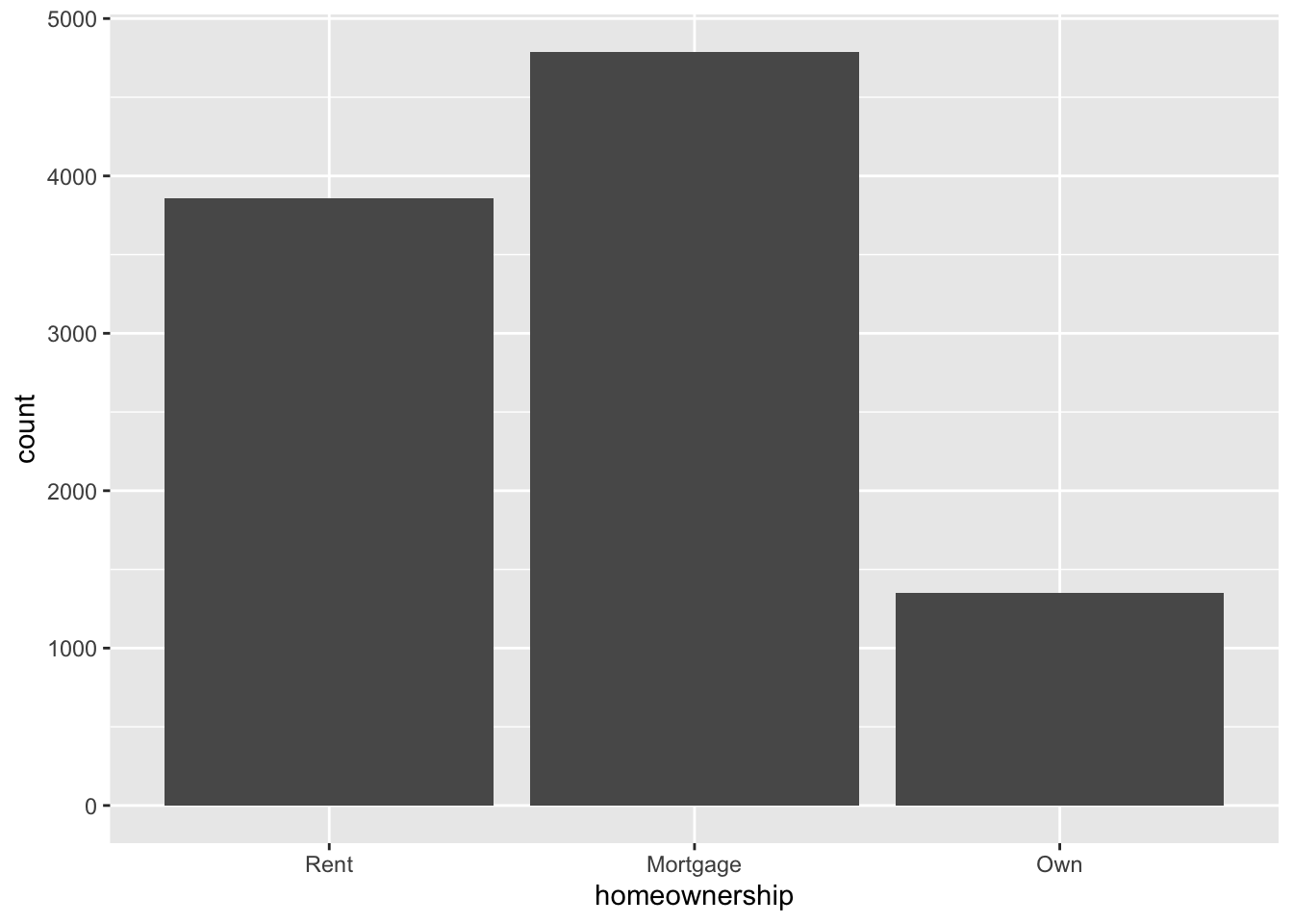
ggplot(loans, aes(x = homeownership)) +
  geom_bar()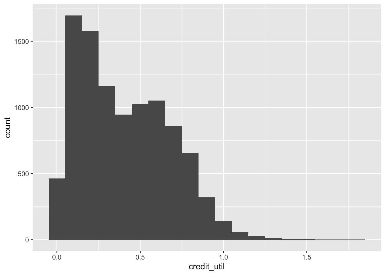

Interest rate vs. credit utilization

For a regression model for predicting interest rate from credit utilization. Display the summary output.

rate_util_fit <- linear_reg() |>
  fit(interest_rate ~ credit_util, data = loans)

tidy(rate_util_fit)

# A tibble: 2 × 5
  term        estimate std.error statistic   p.value
  <chr>          <dbl>     <dbl>     <dbl>     <dbl>
1 (Intercept)    10.5     0.0871     121.  0        
2 credit_util     4.73    0.180       26.3 1.18e-147

Visualize the model.

ggplot(loans, aes(x = credit_util, y = interest_rate)) +
  geom_point(alpha = 0.5) +
  geom_smooth(method = "lm")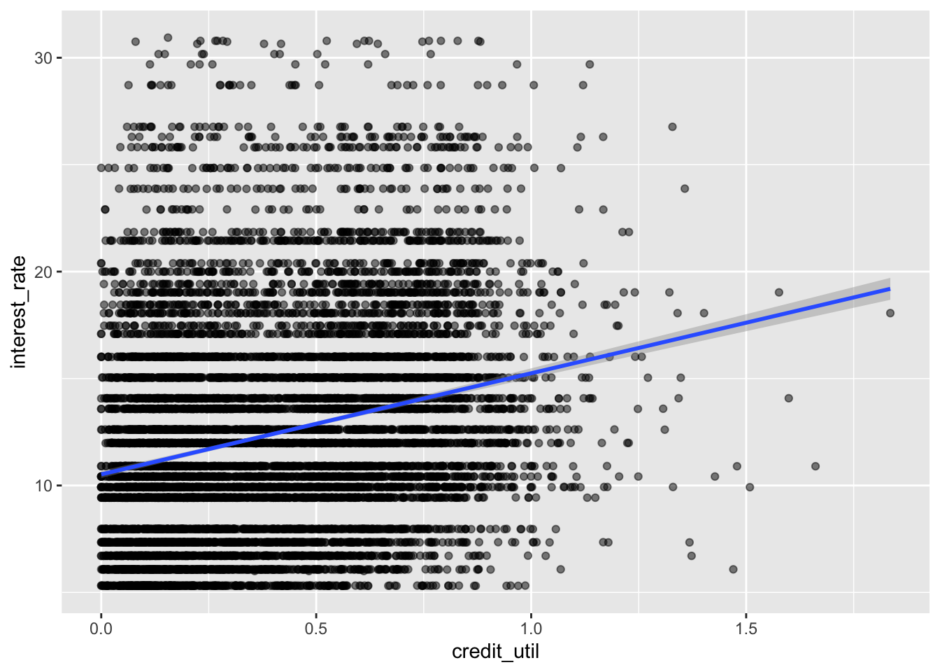

Interpret the intercept and the slope.

Intercept: Borrowers with 0 credit utilization are predicted, on average, to get an interest rate of 10.5%.

Slope: For each additional point credit utilization is higher, interest rate is predicted to be higher, on average, by 4.73%.

Interest rate vs. homeownership

Fit a regression model for predicting interest rate from homeownership and display the summary output.

rate_home_fit <- linear_reg() |>
  fit(interest_rate ~ homeownership, data = loans)

tidy(rate_home_fit)

# A tibble: 3 × 5
  term                  estimate std.error statistic  p.value
  <chr>                    <dbl>     <dbl>     <dbl>    <dbl>
1 (Intercept)             12.9      0.0803    161.   0       
2 homeownershipMortgage   -0.866    0.108      -8.03 1.08e-15
3 homeownershipOwn        -0.611    0.158      -3.88 1.06e- 4

Interpret each coefficient in context of the problem.
- Intercept: Loan applicants who rent are predicted to receive an interest rate of 12.9%, on average.
- Slopes:
  - The model predicts that loan applicants who have a mortgage for their home receive 0.866% lower interest rate than those who rent their home, on average.
  - The model predicts that loan applicants who own their home receive 0.611% lower interest rate than those who rent their home, on average.

Interest rate vs. credit utilization and homeownership

Main effects model

Fit a regression model to predict interest rate from credit utilization and homeownership, without an interaction effect between the two predictors. Display the summary output.

rate_util_home_fit <- linear_reg() |>
  fit(interest_rate ~ credit_util + homeownership, data = loans)

tidy(rate_util_home_fit)

# A tibble: 4 × 5
  term                  estimate std.error statistic   p.value
  <chr>                    <dbl>     <dbl>     <dbl>     <dbl>
1 (Intercept)              9.93      0.140    70.8   0        
2 credit_util              5.34      0.207    25.7   2.20e-141
3 homeownershipMortgage    0.696     0.121     5.76  8.71e-  9
4 homeownershipOwn         0.128     0.155     0.827 4.08e-  1

Write the estimated regression equation for loan applications from each of the homeownership groups separately.
- Rent: \(\widehat{interest~rate} = 9.93 + 5.34 \times credit~util\)
- Mortgage: \(\widehat{interest~rate} = 10.626 + 5.34 \times credit~util\)
- Own: \(\widehat{interest~rate} = 10.058 + 5.34 \times credit~util\)
How does the model predict the interest rate to vary as credit utilization varies for loan applicants with different homeownership status. Are the rates the same or different?

The same.

Interaction effects model

Fit a regression model to predict interest rate from credit utilization and homeownership, with an interaction effect between the two predictors. Display the summary output.

rate_util_home_int_fit <- linear_reg() |>
  fit(interest_rate ~ credit_util * homeownership, data = loans)

tidy(rate_util_home_int_fit)

# A tibble: 6 × 5
  term                              estimate std.error statistic  p.value
  <chr>                                <dbl>     <dbl>     <dbl>    <dbl>
1 (Intercept)                          9.44      0.199     47.5  0       
2 credit_util                          6.20      0.325     19.1  1.01e-79
3 homeownershipMortgage                1.39      0.228      6.11 1.04e- 9
4 homeownershipOwn                     0.697     0.316      2.20 2.75e- 2
5 credit_util:homeownershipMortgage   -1.64      0.457     -3.58 3.49e- 4
6 credit_util:homeownershipOwn        -1.06      0.590     -1.80 7.24e- 2

Write the estimated regression equation for loan applications from each of the homeownership groups separately.
- Rent: \(\widehat{interest~rate} = 9.44 + 6.20 \times credit~util\)
- Mortgage: \(\widehat{interest~rate} = 10.83 + 4.56 \times credit~util\)
- Own: \(\widehat{interest~rate} = 10.137 + 5.14 \times credit~util\)
How does the model predict the interest rate to vary as credit utilization varies for loan applicants with different homeownership status. Are the rates the same or different?

Different.

Choosing a model

Rule of thumb: Occam’s Razor - Don’t over-complicate the situation! We prefer the simplest best model.

Display model level summary statistics.

glance(rate_util_home_fit)

# A tibble: 1 × 12
  r.squared adj.r.squared sigma statistic   p.value    df  logLik    AIC    BIC
      <dbl>         <dbl> <dbl>     <dbl>     <dbl> <dbl>   <dbl>  <dbl>  <dbl>
1    0.0682        0.0679  4.83      244. 1.25e-152     3 -29926. 59861. 59897.
# ℹ 3 more variables: deviance <dbl>, df.residual <int>, nobs <int>

glance(rate_util_home_int_fit)

# A tibble: 1 × 12
  r.squared adj.r.squared sigma statistic   p.value    df  logLik    AIC    BIC
      <dbl>         <dbl> <dbl>     <dbl>     <dbl> <dbl>   <dbl>  <dbl>  <dbl>
1    0.0694        0.0689  4.83      149. 4.79e-153     5 -29919. 59852. 59903.
# ℹ 3 more variables: deviance <dbl>, df.residual <int>, nobs <int>

What is R-squared? What is adjusted R-squared?

R-squared is the percent variability in the response that is explained by our model. (Can use when models have same number of variables for model selection)

Adjusted R-squared is similar, but has a penalty for the number of variables in the model. (Should use for model selection when models have different numbers of variables).

Based on the adjusted \(R^2\)s of these two models, which one do we prefer?

The interaction effects model, though just barely.

Another model to consider

Let’s add one more model to the variable – issue month. Should we add this variable to the interaction effects model from earlier?

linear_reg() |>
  fit(interest_rate ~ credit_util * homeownership + issue_month, data = loans) |>
  glance()

# A tibble: 1 × 12
  r.squared adj.r.squared sigma statistic   p.value    df  logLik    AIC    BIC
      <dbl>         <dbl> <dbl>     <dbl>     <dbl> <dbl>   <dbl>  <dbl>  <dbl>
1    0.0694        0.0688  4.83      106. 5.62e-151     7 -29919. 59856. 59921.
# ℹ 3 more variables: deviance <dbl>, df.residual <int>, nobs <int>

No, the adjusted R-squared goes down.