Bootstrapping Duke Forest houses (Complete)

In this code along, we will use bootstrapping to construct confidence intervals.

Packages

We will use tidyverse and tidymodels for data exploration and modeling, respectively, and the openintro package for the data.

library(tidyverse)
library(tidymodels)
library(openintro)

Data

The data are on houses that were sold in the Duke Forest neighborhood of Durham, NC around November 2020. It was originally scraped from Zillow, and can be found in the duke_forest data set in the openintro R package.

glimpse(duke_forest)

Rows: 98
Columns: 13
$ address    <chr> "1 Learned Pl, Durham, NC 27705", "1616 Pinecrest Rd, Durha…
$ price      <dbl> 1520000, 1030000, 420000, 680000, 428500, 456000, 1270000, …
$ bed        <dbl> 3, 5, 2, 4, 4, 3, 5, 4, 4, 3, 4, 4, 3, 5, 4, 5, 3, 4, 4, 3,…
$ bath       <dbl> 4.0, 4.0, 3.0, 3.0, 3.0, 3.0, 5.0, 3.0, 5.0, 2.0, 3.0, 3.0,…
$ area       <dbl> 6040, 4475, 1745, 2091, 1772, 1950, 3909, 2841, 3924, 2173,…
$ type       <chr> "Single Family", "Single Family", "Single Family", "Single …
$ year_built <dbl> 1972, 1969, 1959, 1961, 2020, 2014, 1968, 1973, 1972, 1964,…
$ heating    <chr> "Other, Gas", "Forced air, Gas", "Forced air, Gas", "Heat p…
$ cooling    <fct> central, central, central, central, central, central, centr…
$ parking    <chr> "0 spaces", "Carport, Covered", "Garage - Attached, Covered…
$ lot        <dbl> 0.97, 1.38, 0.51, 0.84, 0.16, 0.45, 0.94, 0.79, 0.53, 0.73,…
$ hoa        <chr> NA, NA, NA, NA, NA, NA, NA, NA, NA, NA, NA, NA, NA, NA, NA,…
$ url        <chr> "https://www.zillow.com/homedetails/1-Learned-Pl-Durham-NC-…

Model

Fit a linear model predicting price of houses from their area.

df_fit <- linear_reg() |>
  fit(price ~ area, data = duke_forest)

tidy(df_fit)

# A tibble: 2 × 5
  term        estimate std.error statistic  p.value
  <chr>          <dbl>     <dbl>     <dbl>    <dbl>
1 (Intercept)  116652.   53302.       2.19 3.11e- 2
2 area            159.      18.2      8.78 6.29e-14

Bootstrap confidence interval

Calculate the observed fit (slope):

observed_fit <- duke_forest |>
  specify(price ~ area) |>
  fit()

observed_fit

# A tibble: 2 × 2
  term      estimate
  <chr>        <dbl>
1 intercept  116652.
2 area          159.

Take n bootstrap samples and fit models to each one:

n = 100
set.seed(20241115)

boot_fits <- duke_forest |>
  specify(price ~ area) |>
  generate(reps = n, type = "bootstrap") |>
  fit()

boot_fits

# A tibble: 200 × 3
# Groups:   replicate [100]
   replicate term      estimate
       <int> <chr>        <dbl>
 1         1 intercept  149083.
 2         1 area          143.
 3         2 intercept  226037.
 4         2 area          110.
 5         3 intercept   37464.
 6         3 area          188.
 7         4 intercept    7631.
 8         4 area          208.
 9         5 intercept  245406.
10         5 area          104.
# ℹ 190 more rows

Why do we set a seed before taking the bootstrap samples?

To get the same random samples each time we run the code / render the document.

Make a histogram of the bootstrap samples to visualize the bootstrap distribution.

boot_fits |>
  filter(term == "area") |>
  ggplot(aes(x = estimate)) +
  geom_histogram()

`stat_bin()` using `bins = 30`. Pick better value with `binwidth`.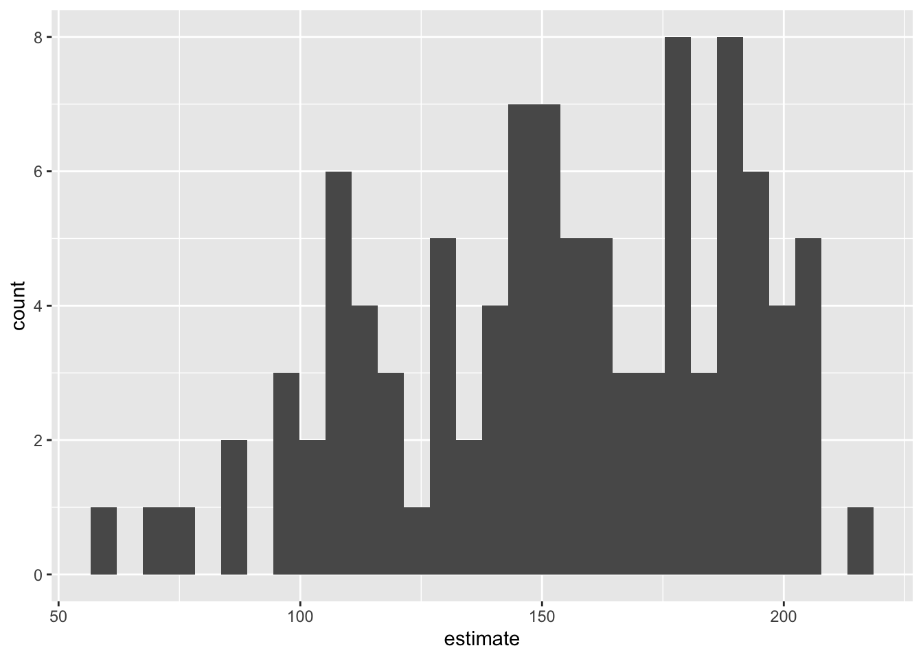

Compute the 95% confidence interval as the middle 95% of the bootstrap distribution:

get_confidence_interval(
  boot_fits, 
  point_estimate = observed_fit, 
  level = 0.95,
  type = "percentile"
)

# A tibble: 2 × 3
  term      lower_ci upper_ci
  <chr>        <dbl>    <dbl>
1 area          79.9     207.
2 intercept  -3694.   316939.

Changing confidence level

Modify the code from Step 3 to create a 90% confidence interval.

get_confidence_interval(
  boot_fits, 
  point_estimate = observed_fit, 
  level = 0.90,
  type = "percentile"
)

# A tibble: 2 × 3
  term      lower_ci upper_ci
  <chr>        <dbl>    <dbl>
1 area          94.7     203.
2 intercept   8234.   284161.

Modify the code from Step 3 to create a 99% confidence interval.

get_confidence_interval(
  boot_fits, 
  point_estimate = observed_fit, 
  level = 0.99,
  type = "percentile"
)

# A tibble: 2 × 3
  term      lower_ci upper_ci
  <chr>        <dbl>    <dbl>
1 area          64.2     211.
2 intercept -19831.   370166.

Which confidence level produces the most accurate confidence interval (90%, 95%, 99%)? Explain.

99%, widest.

Which confidence level produces the most precise confidence interval (90%, 95%, 99%)? Explain

90%, narrowest.

If we want to be very certain that we capture the population parameter, should we use a wider or a narrower interval? What drawbacks are associated with using a wider interval?

Wider, but then it’s less informative.