Predicting income level with logistic regression
Modeling Inference
Data Science with R
Getting started
Programming exercises are designed to provide an opportunity for you to put what you learn in the videos and readings. These exercises feature interactive code cells which allow you to write, edit, and run R code without leaving your browser.
When the ▶️ Run Code button turns to a solid color (with no flashing bubble indicating that the document is still loading), you can interact with the code cells!
Packages
We’ll use the tidyverse and tidymodels for this programming exercise. These are already installed for you to use!
Motivation
Census data can help us predict income based on other variables, such as demographic, social, and economic variables. We can use this information to help gain deeper insights into the economic well-being of a population, which can help practically inform items such as strategic planning, and market analysis. In this programming exercise, we are going to explore the relationship between different predictors, and if an individual was making more or less than $50,000 USD a year in 1994 in the United States.
Data
The dataset we will be using for this exercise is from the 1994 Census database, extracted by Barry Becker. These data can be found on the UCI Machine Learning Repository. Expand the tab below to look at the data key. In the code chunk below, we change income to be a factor. Our outcome variable needs to be a factor in order to fit a logistic regression model.
CautionData dictionary
| Variable Name | Description |
| age | Age |
| workclass | Private, Self-emp-not-inc, Self-emp-inc, Federal-gov, Local-gov, State-gov, Without-pay, Never-worked. |
| education | Bachelors, Some-college, 11th, HS-grad, Prof-school, Assoc-acdm, Assoc-voc, 9th, 7th-8th, 12th, Masters, 1st-4th, 10th, Doctorate, 5th-6th, Preschool. |
| education-num | Education Level as a number |
| marital-status | Married-civ-spouse, Divorced, Never-married, Separated, Widowed, Married-spouse-absent, Married-AF-spouse. |
| occupation | Tech-support, Craft-repair, Other-service, Sales, Exec-managerial, Prof-specialty, Handlers-cleaners, Machine-op-inspect, Adm-clerical, Farming-fishing, Transport-moving, Priv-house-serv, Protective-serv, Armed-Forces. |
| relationship | Wife, Own-child, Husband, Not-in-family, Other-relative, Unmarried. |
| race | White, Asian-Pac-Islander, Amer-Indian-Eskimo, Other, Black. |
| sex | Female, Male. |
| native-country | United-States, Cambodia, England, Puerto-Rico, Canada, Germany, Outlying-US(Guam-USVI-etc), India, Japan, Greece, South, China, Cuba, Iran, Honduras, Philippines, Italy, Poland, Jamaica, Vietnam, Mexico, Portugal, Ireland, France, Dominican-Republic, Laos, Ecuador, Taiwan, Haiti, Columbia, Hungary, Guatemala, Nicaragua, Scotland, Thailand, Yugoslavia, El-Salvador, Trinadad&Tobago, Peru, Hong, Holand-Netherlands. |
| income | >50K, <=50K. |
Exploratory data analysis
Before we fit a logistic regression model, we are going to explore these data. Let’ start with exploring the outcome variable of interest, cholesterol (income). For this exercise, we are going to investigate the relationship between income and age.
Let’s calculate the mean and sd of age for each level of income. What does this tell us? When fitting a logistic regression model, would we expect the probability of making more than $50,000 to increase or decrease as you get older?
TipSolution
# A tibble: 2 × 3
  income mean_age sd_age
  <fct>     <dbl>  <dbl>
1 <=50K      36.8   14.0
2 >50K       44.2   10.5
The mean age for those making less than $50,000 is roughly 7.4 years younger than the mean age of those making more than $50,000. The spread (standard deviation) is also higher for those making less than $50,000 in comparison to those making more.
Based on this information, we would expect the probability of making more than $50,000 to increase as age increases.
Modeling
The variable income in our dataset is changed to a fct, with the first level being of this factor being <=50K, and second level being >50K. Because of this ordering, we are going to be modeling the log-odds/probability of >50K. The default in tidymodels code for logistic regression is to treat the second level factor as our success.
Fit a logistic regression model below with income as the outcome and age as the predictor. Compare your output model defined below. Is the outcome the log-odds of making more than $50,000 or the probability of making more that $50,000?
\[ \log \left( \frac{p}{1-p} \right) = -2.74 + 0.0395(\text{age}) \]
TipSolution
income_model <- logistic_reg() |>
  fit(income ~ age, data = income, family = binomial)

tidy(income_model)
# A tibble: 2 × 5
term estimate std.error statistic p.value
<chr> <dbl> <dbl> <dbl> <dbl>
1 (Intercept) -2.74 0.0427 -64.2 0
2 age 0.0395 0.000967 40.9 0The logistic regression model we fit models the log-odds: \[\log \left( \frac{p}{1-p} \right)\], where p represents the probability of of making more than $50,000.
Probabilities
To model the probability of making more than $50,000, we need to expoentiate both sides of the eqaution. See below:
\[ p = \frac{e^{-2.74 + 0.0395(\text{age})}}{1 + e^{-2.74 + 0.0395(\text{age})}} \]
Using your model, what’s the probability of making more than $50,000 if you are 60 years old in 1994?
TipSolution
\[ p = \frac{e^{-2.74 + 0.0395(\text{60})}}{1 + e^{-2.74 + 0.0395(\text{60})}} = 0.408 \]
We can also find this in R!
age_predict <- tibble(age = 60)

predict(income_model, age_predict, type = "prob")
# A tibble: 1 × 2
`.pred_<=50K` `.pred_>50K`
<dbl> <dbl>
1 0.592 0.408Based on your conclusion from your exploratory analysis, does the probability of making over $50,000 increase or decrease as you age? How can you tell from your model?
TipSolution
The coefficient associated with age is positive, meaning that the estimated probability of making more than $50,000 increases as age increases.
We can further show your intuition is correct by calculating the probability at the age of 61, and see if the difference between the probability at the age of 60 is positive or negative.
\(p = \frac{e^{-2.74 + 0.0395(\text{61})}}{1 + e^{-2.74 + 0.0395(\text{61})}} = 0.418\)
0.418 - 0.408 = 0.01
The estimated probability of making more than $50,000 increases by roughly 1 percent as you go from age 60 to 61.
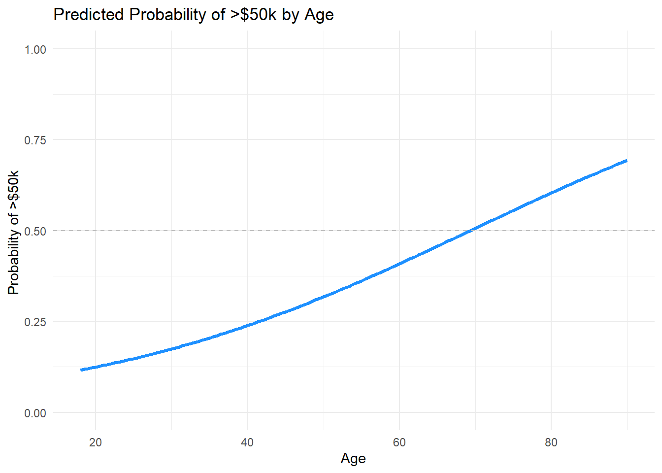
Because this is not linear regression, the estimated change in probability of making more than 50,000 USD at the age of 60 to 61 is NOT the same as other one-year age differences. Explore this using the code below (ex. calculate the probability of making more than 50,000 USD at the age of 20 versus 21). Compare it to the visualization above.
Summary
We can use a logistic regression model to estimate the log-odds/probability of success of the outcome variable.
The outcome variable must be binary and encoded as a factor.
We start the model fit with
logistic_reg()instead oflinear_reg().
Your turn: Challenge
There are many other variables that could explain the probability of making more than $50,000 than just age in 1994. Now, we challenge you to fit a more complicated model to help better understand our variable of interest, income.