Language of models

Modeling and inference

Data Science with R

What is a model?

Modeling

Use models to explain the relationship between variables and to make predictions
For now we will focus on linear models (but remember there are many many other types of models too!)

Modeling

Modeling cars

What is the relationship between cars’ weights and their mileage?
What is your best guess for a car’s MPG that weighs 3,500 pounds?

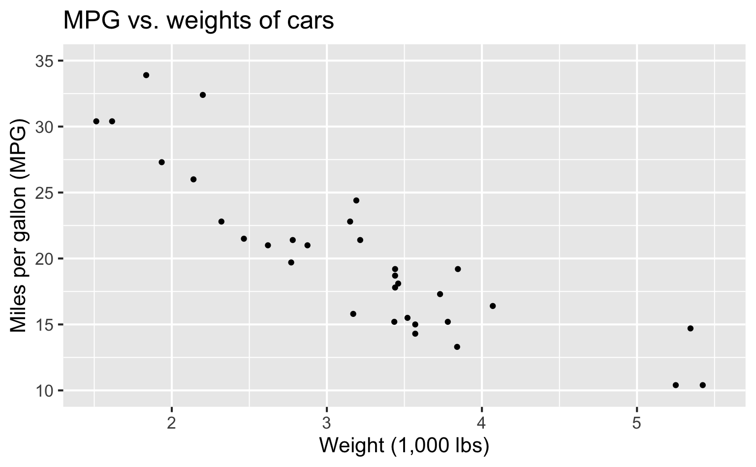
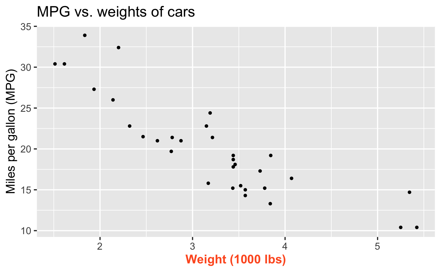
Modelling cars

Describe: What is the relationship between cars’ weights and their mileage?

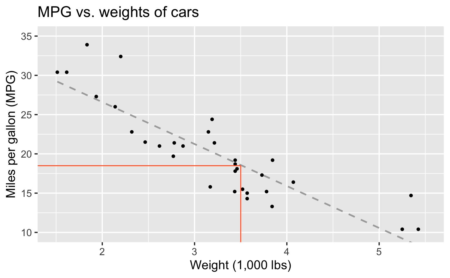
Modelling cars

Predict: What is your best guess for a car’s MPG that weighs 3,500 pounds?

Modeling

Use models to explain the relationship between variables and to make predictions
For now we will focus on linear models (but there are many many other types of models too!)

Modeling vocabulary

Outcome: Variable whose behavior or variation you are trying to understand, on the y-axis (aka response variable, dependent variable)
Predictor(s): Other variable(s) that you want to use to explain the variation in the outcome, on the x-axis (aka explanatory variable(s), independent variable(s))
Model function: The regression line for predicting the outcome variable from the predictor variable(s), comprised generally of an intercept and a slope for each predictor
Predicted value: Output of the model function, which gives the typical (expected) value of the outcome conditioning on the predictor
Residuals: A measure of how far each case’s observed value is from its predicted value (based on a particular model)
- Residual = Observed value - Predicted value
- Tells how far above/below the expected value each case is

Predictor

mpg	wt
21	2.62
21	2.875
22.8	2.32
21.4	3.215
18.7	3.44
18.1	3.46
...	...

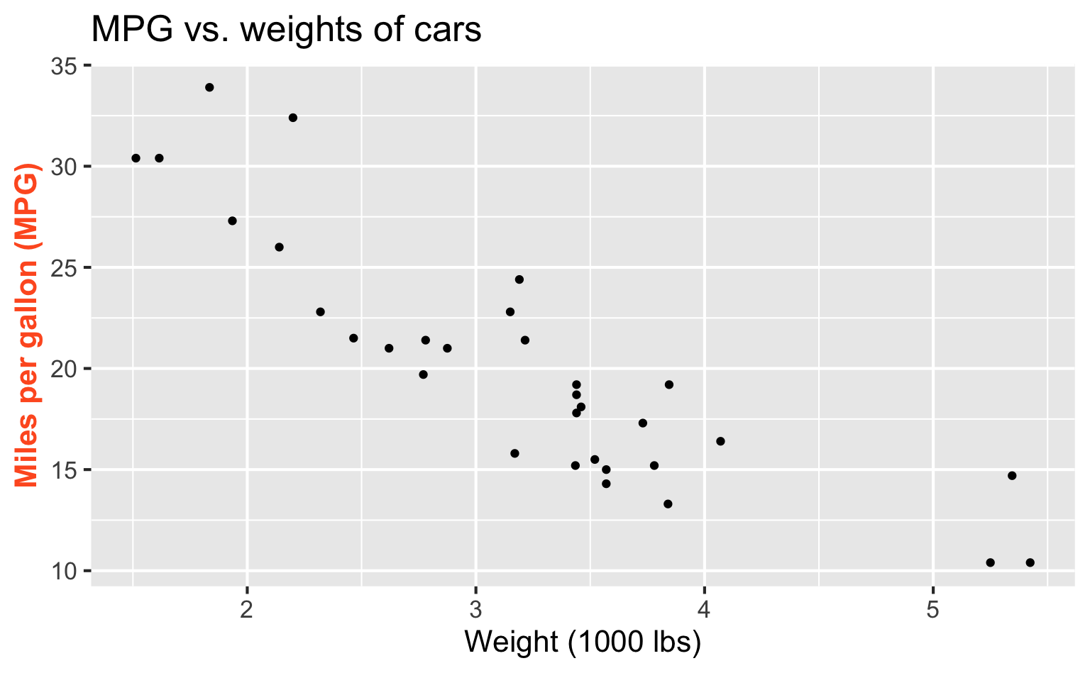
Outcome

mpg	wt
21	2.62
21	2.875
22.8	2.32
21.4	3.215
18.7	3.44
18.1	3.46
...	...

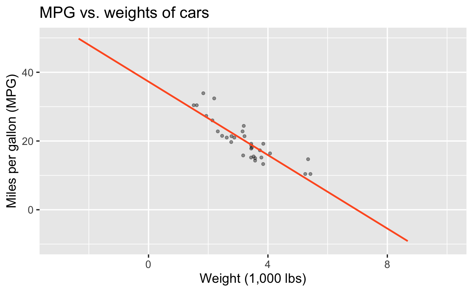
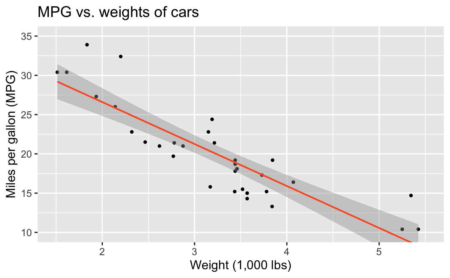
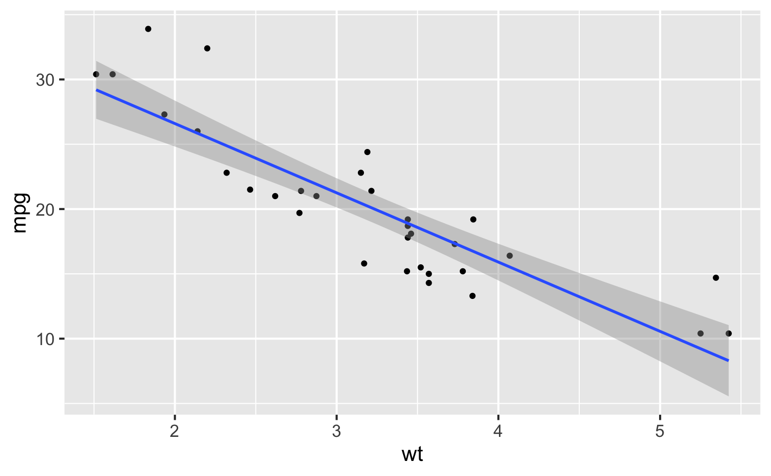
Regression line

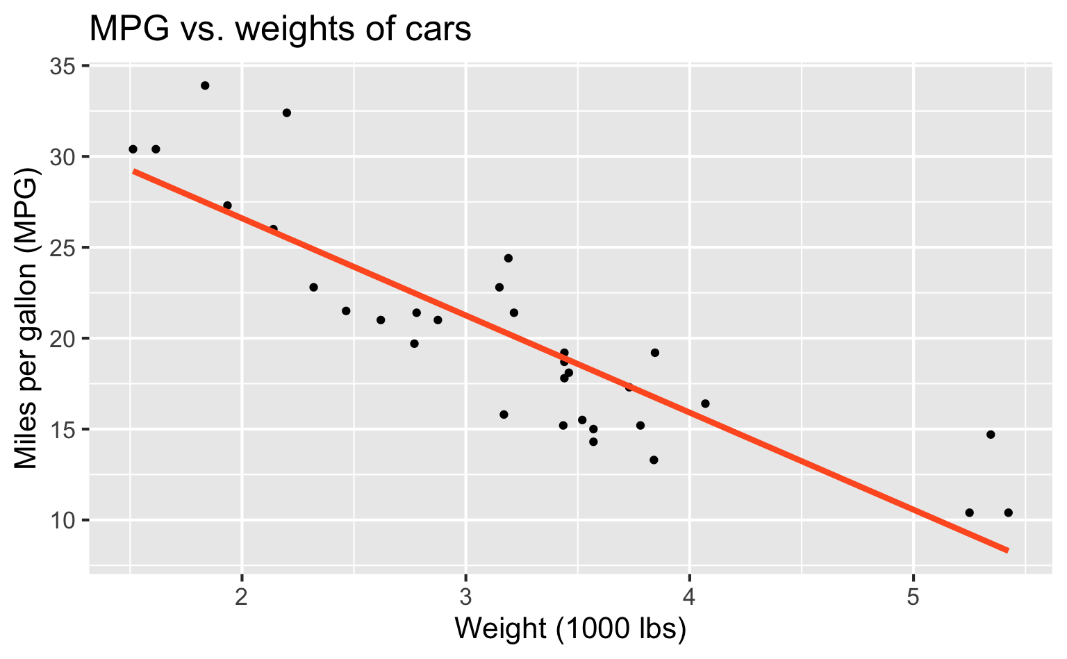
Regression line: slope

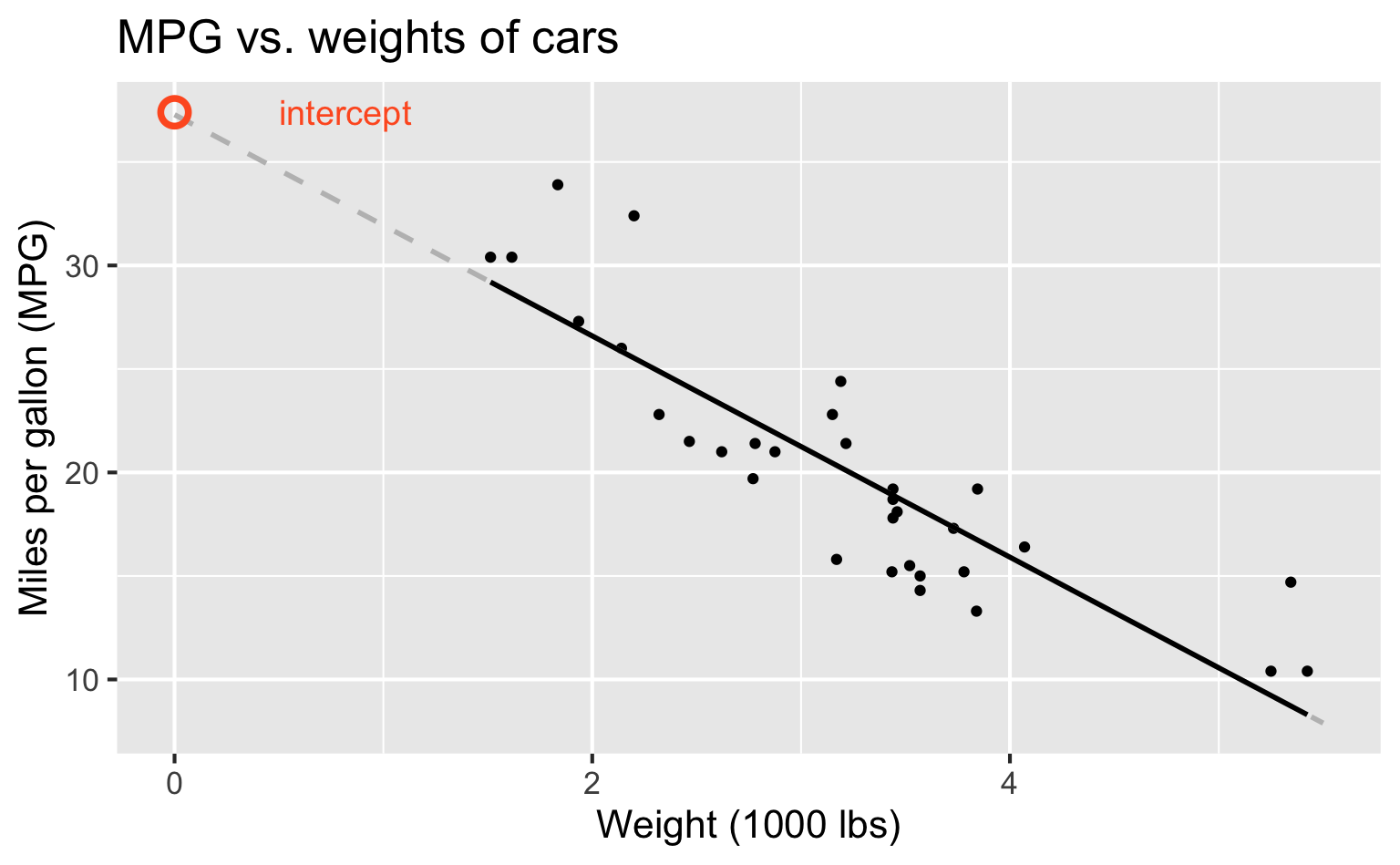
Regression line: intercept

Correlation

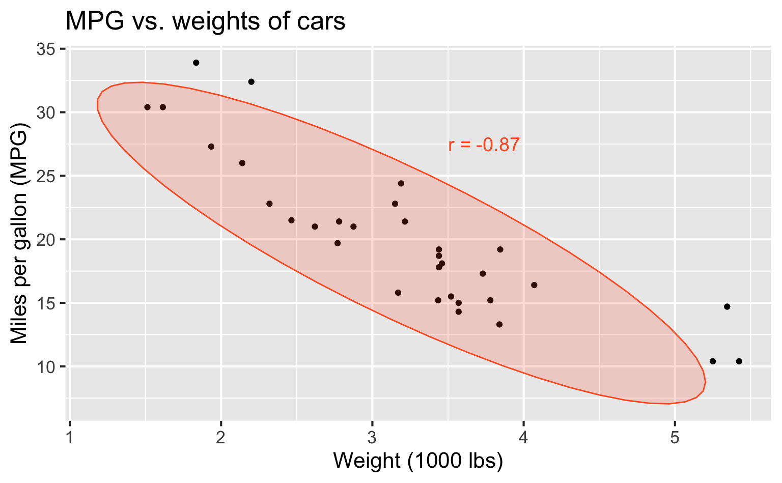
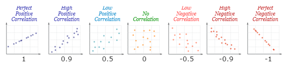
Correlation

Ranges between -1 and 1.
Same sign as the slope.

Visualizing the model

ggplot(mtcars, aes(x = wt, y = mpg)) +
  geom_point() +
  geom_smooth(method = "lm")

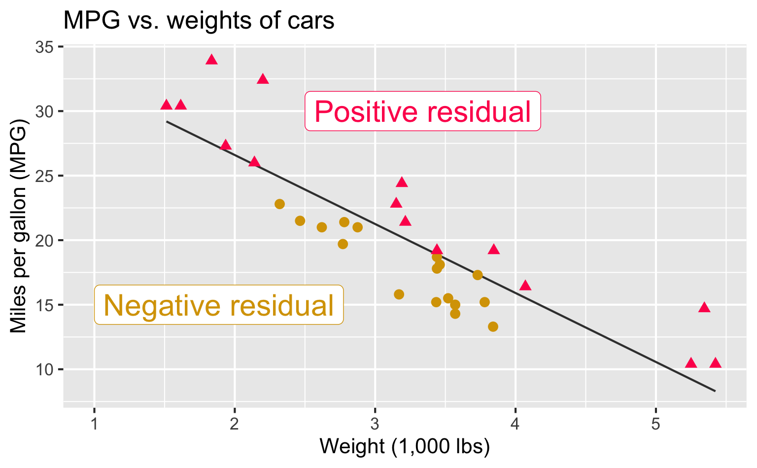
Residuals

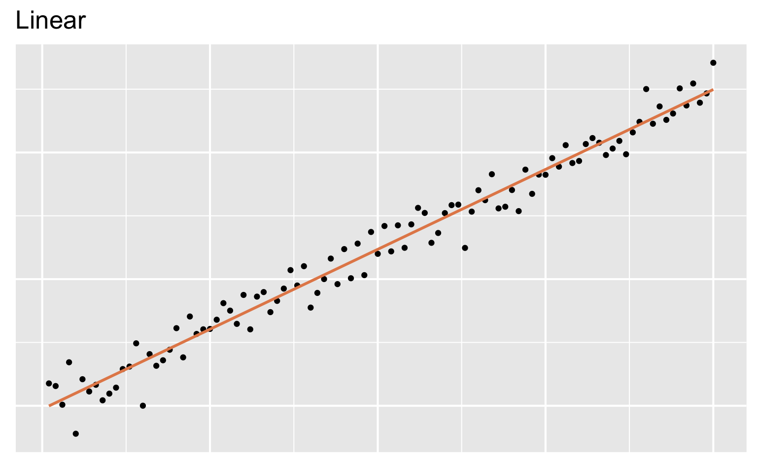
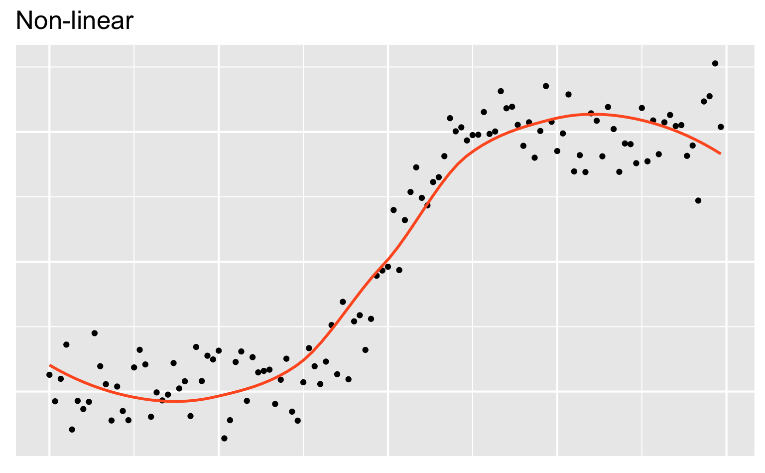
Extending regression lines

Models - upsides and downsides

Models can sometimes reveal patterns that are not evident in a graph of the data. This is a great advantage of modeling over simple visual inspection of data.
There is a real risk, however, that a model is imposing structure that is not really there on the scatter of data, just as people imagine animal shapes in the stars. A skeptical approach is always warranted.

Variation around the model…

is just as important as the model, if not more!

Statistics is the explanation of variation in the context of what remains unexplained.

The scatter suggests that there might be other factors that account for large parts of painting-to-painting variability, or perhaps just that randomness plays a big role.
Adding more explanatory variables to a model can sometimes usefully reduce the size of the scatter around the model. (We’ll talk more about this later.)

How do we use models?

Predict / classify: Plug in the value(s) of predictor(s) to the model to obtain the predicted value of the outcome
Describe: Quantify the relationship between predictor(s) and outcome with slopes

Predict / classify

How do self-driving cars decide whether an object in front of them is a human, another car, or a trash can?
How does an online shopping website decide which ad to serve to you for the next item you might purchase?
What happens if either of these get it wrong?

Describe

Leisure, commute, physical activity and BP

Relation Between Leisure Time, Commuting, and Occupational Physical Activity With Blood Pressure in 125,402 Adults: The Lifelines Cohort

Byambasukh, Oyuntugs, Harold Snieder, and Eva Corpeleijn. “Relation between leisure time, commuting, and occupational physical activity with blood pressure in 125 402 adults: the lifelines cohort.” Journal of the American Heart Association 9.4 (2020): e014313.

Leisure, commute, physical activity and BP

Background: Whether all domains of daily‐life moderate‐to‐vigorous physical activity (MVPA) are associated with lower blood pressure (BP) and how this association depends on age and body mass index remains unclear.

Methods and Results: In the population‐based Lifelines cohort (N=125,402), MVPA was assessed by the Short Questionnaire to Assess Health‐Enhancing Physical Activity, a validated questionnaire in different domains such as commuting, leisure‐time, and occupational PA. BP was assessed using the last 3 of 10 measurements after 10 minutes’ rest in the supine position. Hypertension was defined as systolic BP ≥140 mm Hg and/or diastolic BP ≥90 mm Hg and/or use of antihypertensives. In regression analysis, higher commuting and leisure‐time but not occupational MVPA related to lower BP and lower hypertension risk. Commuting‐and‐leisure‐time MVPA was associated with BP in a dose‐dependent manner. β Coefficients (95% CI) from linear regression analyses were −1.64 (−2.03 to −1.24), −2.29 (−2.68 to −1.90), and finally −2.90 (−3.29 to −2.50) mm Hg systolic BP for the low, middle, and highest tertile of MVPA compared with “No MVPA” as the reference group after adjusting for age, sex, education, smoking and alcohol use. Further adjustment for body mass index attenuated the associations by 30% to 50%, but more MVPA remained significantly associated with lower BP and lower risk of hypertension. This association was age dependent. β Coefficients (95% CI) for the highest tertiles of commuting‐and‐leisure‐time MVPA were −1.67 (−2.20 to −1.15), −3.39 (−3.94 to −2.82) and −4.64 (−6.15 to −3.14) mm Hg systolic BP in adults <40, 40 to 60, and >60 years, respectively.

Conclusions: Higher commuting and leisure‐time but not occupational MVPA were significantly associated with lower BP and lower hypertension risk at all ages, but these associations were stronger in older adults.