Linear regression with a numerical predictor

Modeling and inference

Data Science with R

Packages and data

Packages

fivethirtyeight for data
tidyverse for data wrangling and visualization
tidymodels for modeling

library(fivethirtyeight)
library(tidyverse)
library(tidymodels)

Data prep

Rename Rotten Tomatoes columns as critics and audience
Rename the dataset as movie_scores

movie_scores <- fandango |>
  rename(
    critics = rottentomatoes, 
    audience = rottentomatoes_user
  )

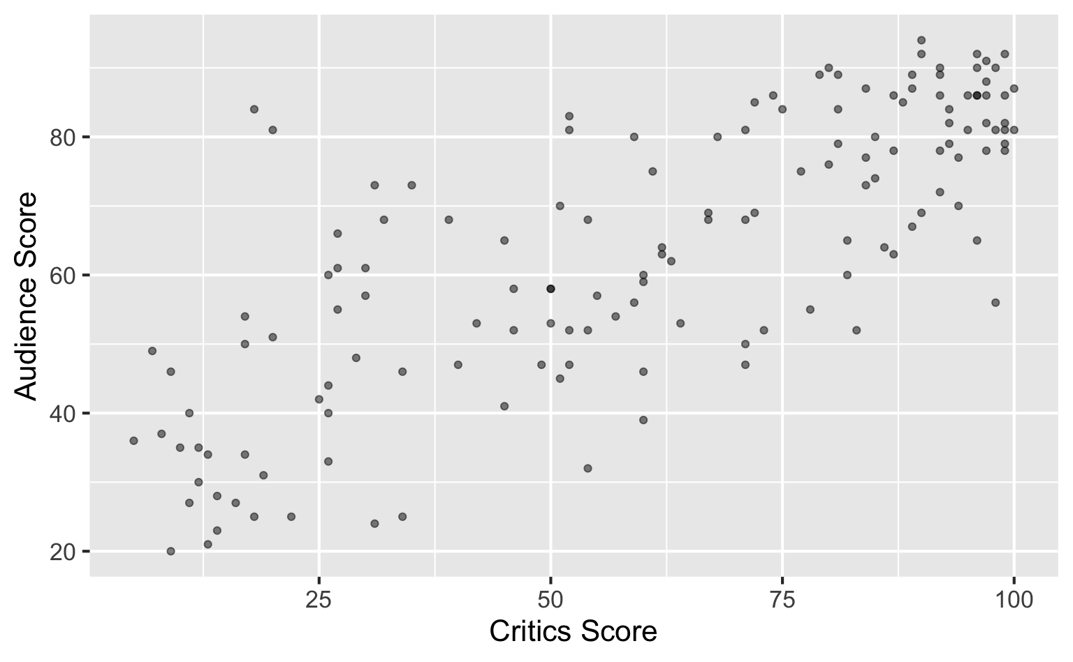
Data overview

movie_scores |>
  select(critics, audience)

# A tibble: 146 × 2
   critics audience
     <int>    <int>
 1      74       86
 2      85       80
 3      80       90
 4      18       84
 5      14       28
 6      63       62
 7      42       53
 8      86       64
 9      99       82
10      89       87
# ℹ 136 more rows

Data visualization

Regression model

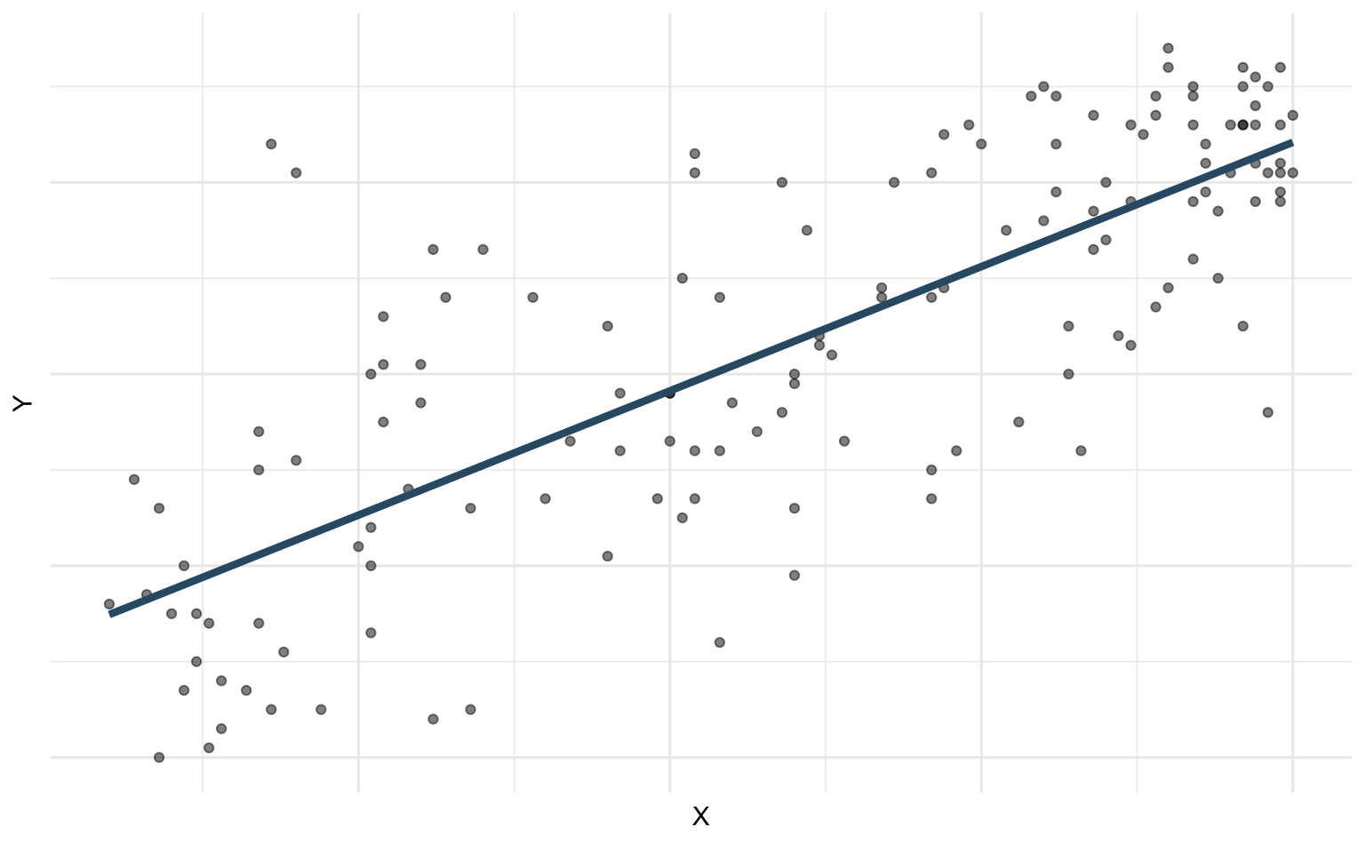
A regression model is a function that describes the relationship between the outcome, \(Y\), and the predictor, \(X\).

\[ \begin{aligned} Y &= \color{black}{\textbf{Model}} + \text{Error} \\[8pt] &= \color{black}{\mathbf{f(X)}} + \epsilon \\[8pt] &= \color{black}{\boldsymbol{\mu_{Y|X}}} + \epsilon \end{aligned} \]

Regression model

\[ \begin{aligned} Y &= \color{#325b74}{\textbf{Model}} + \text{Error} \\[8pt] &= \color{#325b74}{\mathbf{f(X)}} + \epsilon \\[8pt] &= \color{#325b74}{\boldsymbol{\mu_{Y|X}}} + \epsilon \end{aligned} \]

Simple linear regression

Use simple linear regression to model the relationship between a numerical outcome (\(Y\)) and a single numerical predictor (\(X\)): \[\Large{Y = \beta_0 + \beta_1 X + \epsilon}\]

\(\beta_1\): True slope of the relationship between \(X\) and \(Y\)
\(\beta_0\): True intercept of the relationship between \(X\) and \(Y\)
\(\epsilon\): Error (residual)

Simple linear regression

\[ \Large{\hat{Y} = b_0 + b_1 X} \]

\(b_1\): Estimated slope of the relationship between \(X\) and \(Y\)
\(b_0\): Estimated intercept of the relationship between \(X\) and \(Y\)
No error term!

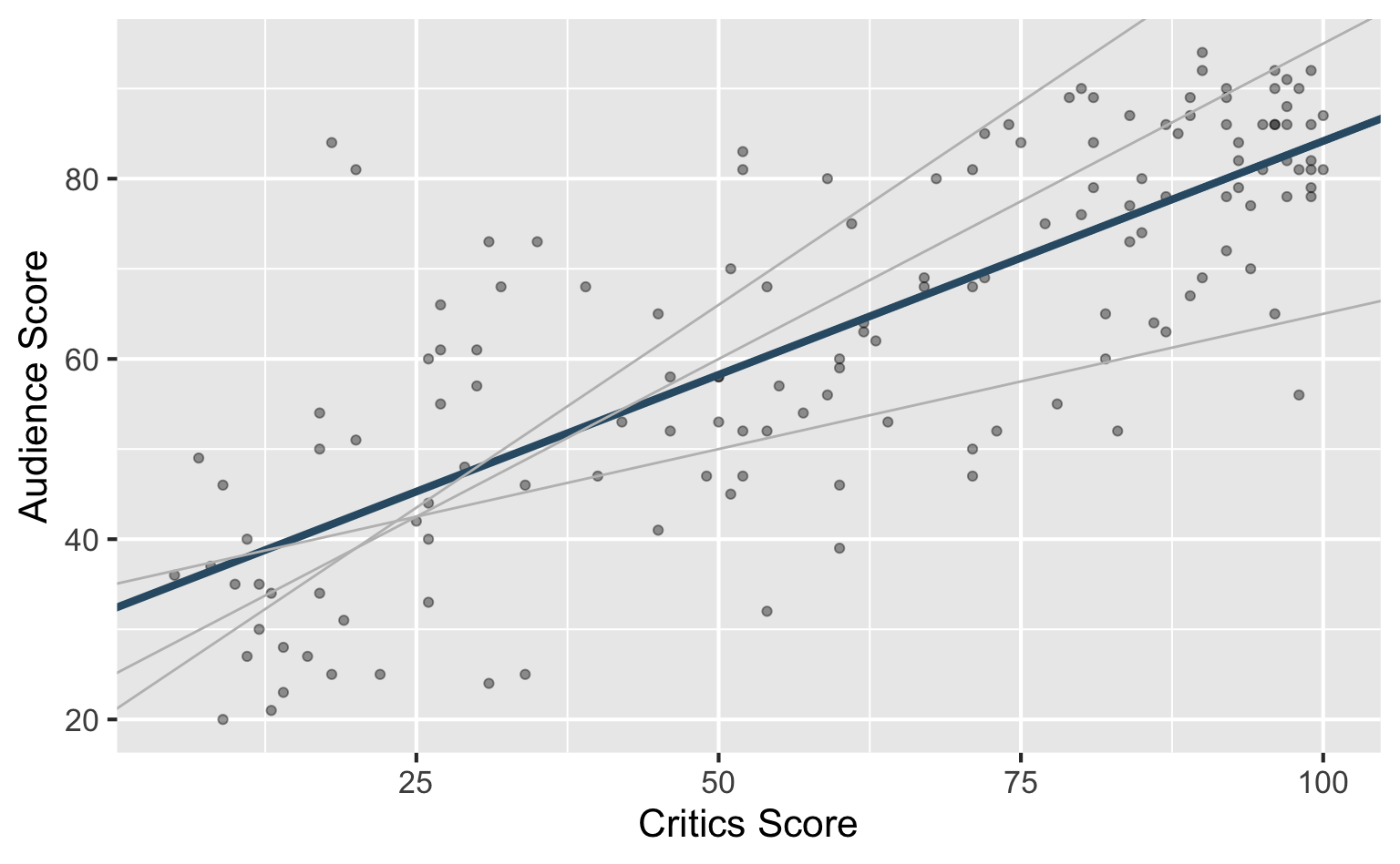
Choosing values for \(b_1\) and \(b_0\)

Residuals

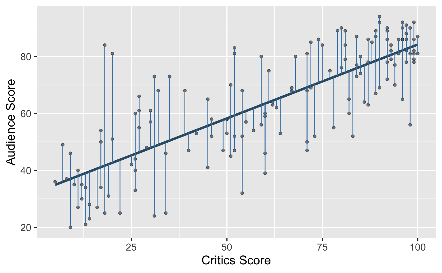
\[ \text{residual} = \text{observed} - \text{predicted} = y - \hat{y} \]

Least squares line

The residual for the \(i^{th}\) observation is

\[ e_i = \text{observed} - \text{predicted} = y_i - \hat{y}_i \]

The sum of squared residuals is

\[ e^2_1 + e^2_2 + \dots + e^2_n \]

The least squares line is the one that minimizes the sum of squared residuals

Fitting a model

movies_fit <- linear_reg() |>
  fit(audience ~ critics, data = movie_scores)

tidy(movies_fit)

# A tibble: 2 × 5
  term        estimate std.error statistic  p.value
  <chr>          <dbl>     <dbl>     <dbl>    <dbl>
1 (Intercept)   32.3      2.34        13.8 4.03e-28
2 critics        0.519    0.0345      15.0 2.70e-31

Interpreting model output

Interpreting the slope

The slope of the model for predicting audience score from critics score is 0.519. Which of the following is the best interpretation of this value?

For every one point increase in the critics score, the audience score goes up by 0.519 points, on average.
For every one point increase in the critics score, we expect the audience score to be higher by 0.519 points, on average.
For every one point increase in the critics score, the audience score goes up by 0.519 points.
For every one point increase in the audience score, the critics score goes up by 0.519 points, on average.

Interpreting the slope

The slope of the model for predicting audience score from critics score is 0.519. Which of the following is the best interpretation of this value?

For every one point increase in the critics score, the audience score goes up by 0.519 points, on average.
For every one point increase in the critics score, we expect the audience score to be higher by 0.519 points, on average.
For every one point increase in the critics score, the audience score goes up by 0.519 points.
For every one point increase in the audience score, the critics score goes up by 0.519 points, on average.

Interpreting slope & intercept

\[ \widehat{\text{audience}} = 32.3 + 0.519 \times \text{critics} \]

Slope: For every one point increase in the critics score, we expect the audience score to be higher by 0.519 points, on average.
Intercept: For movies with a critics score of 0, we expect the audience score to be 32.3 points, on average.

Is the intercept meaningful?

✅ The intercept is meaningful in context of the data if

the predictor can feasibly take values equal to or near zero or
the predictor has values near zero in the observed data

🛑 Otherwise, it might not be meaningful!

Putting it altogether

Least squares regression

The least squares regression line minimizes the sum of squares residuals. It has the following properties:

Goes through the center of mass point (the coordinates corresponding to average \(X\) and average \(Y\)): \(b_0 = \bar{Y} - b_1~\bar{X}\)
Slope of the line has the same sign as the correlation coefficient: \(b_1 = r \frac{s_Y}{s_X}\)
Sum of the residuals is zero: \(\sum_{i = 1}^n \epsilon_i = 0\)
Residuals and \(X\) values are uncorrelated