Linear regression with multiple predictors
Modeling and inference
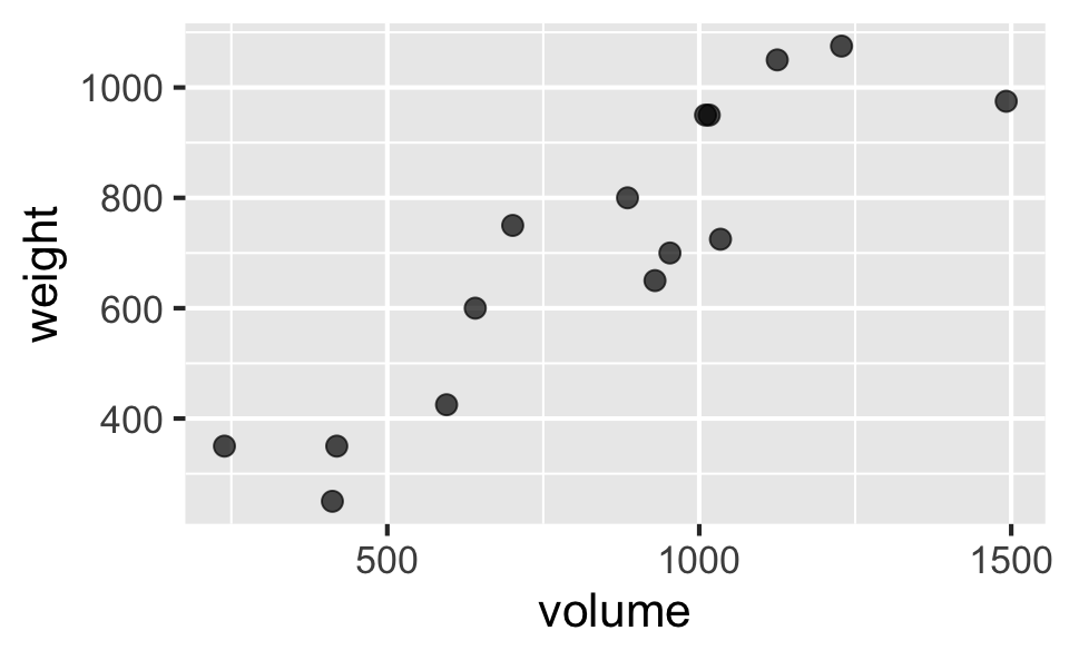
Book weight vs. volume
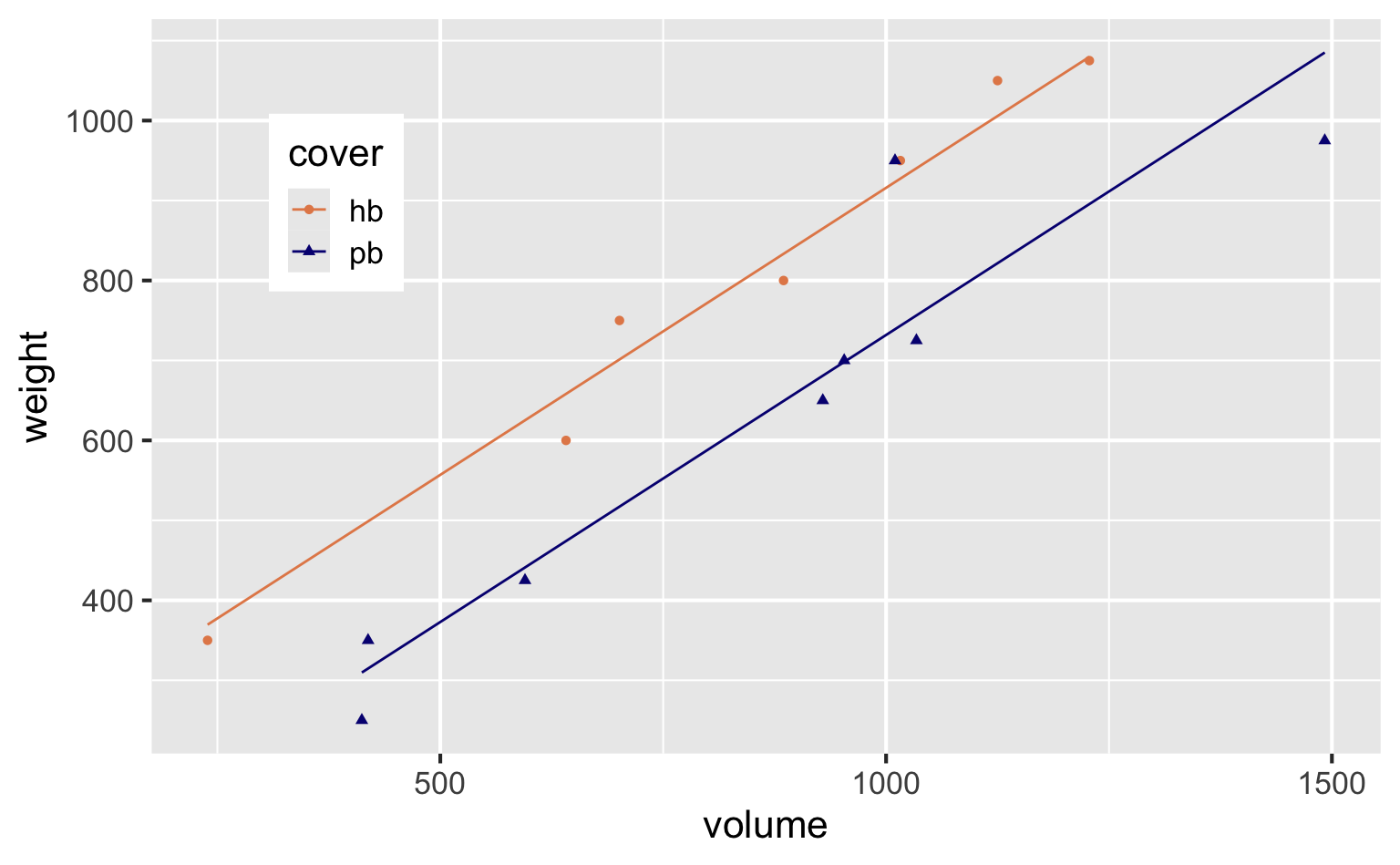
Book weight vs. volume and cover
allbacks_2_fit <- linear_reg() |>
  fit(weight ~ volume + cover, data = allbacks)

tidy(allbacks_2_fit)
# A tibble: 3 × 5
term estimate std.error statistic p.value
<chr> <dbl> <dbl> <dbl> <dbl>
1 (Intercept) 198. 59.2 3.34 0.00584
2 volume 0.718 0.0615 11.7 0.0000000660
3 coverpb -184. 40.5 -4.55 0.000672 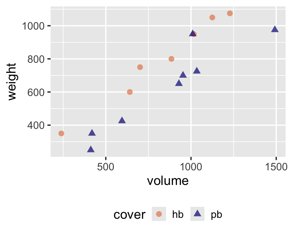
Model 1 - visualized
# A tibble: 1 × 2
  r.squared adj.r.squared
      <dbl>         <dbl>
1     0.803         0.787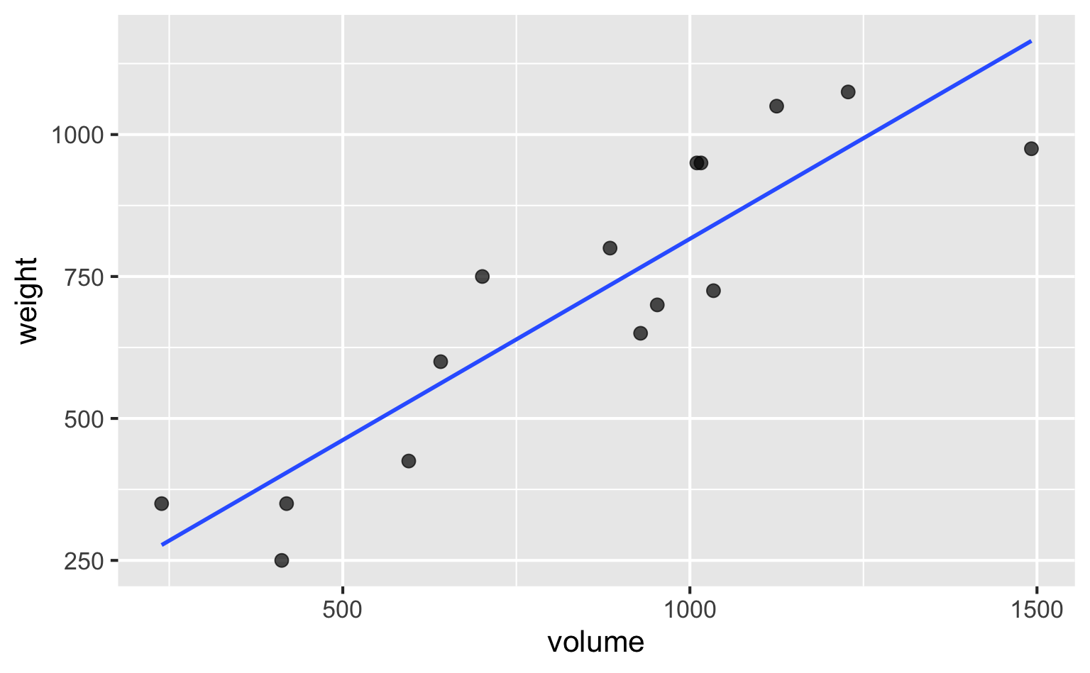
Model 2 - visualized
# A tibble: 1 × 2
  r.squared adj.r.squared
      <dbl>         <dbl>
1     0.927         0.915