Logistic regression
Modeling and inference
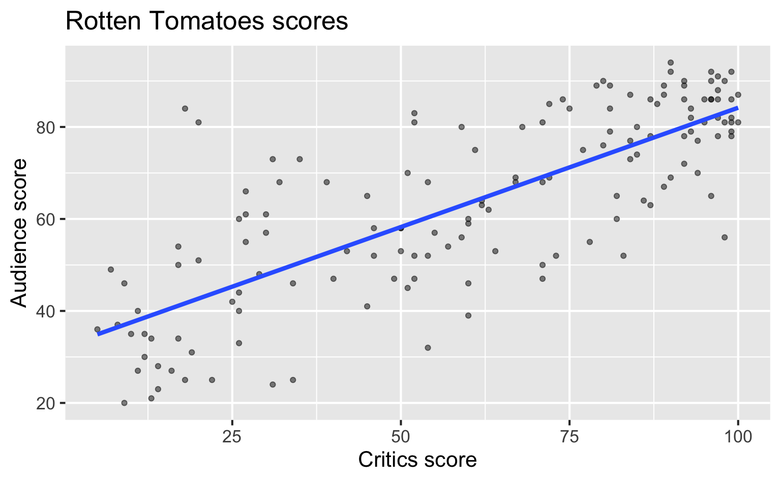
Recap: Simple linear regression
Numerical outcome and one numerical predictor:
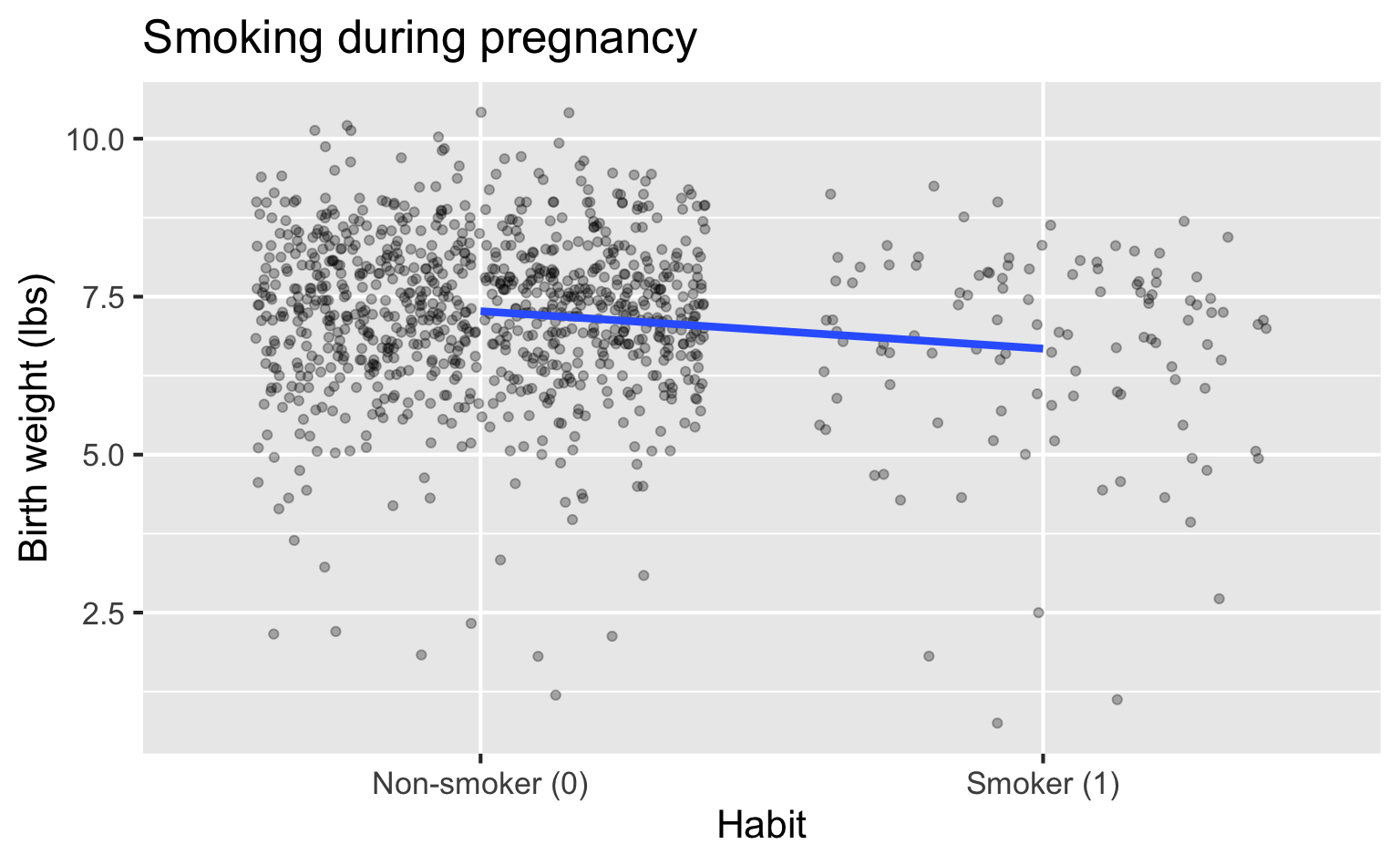
Recap: Multiple linear regression
Numerical outcome and one categorical predictor (two levels):
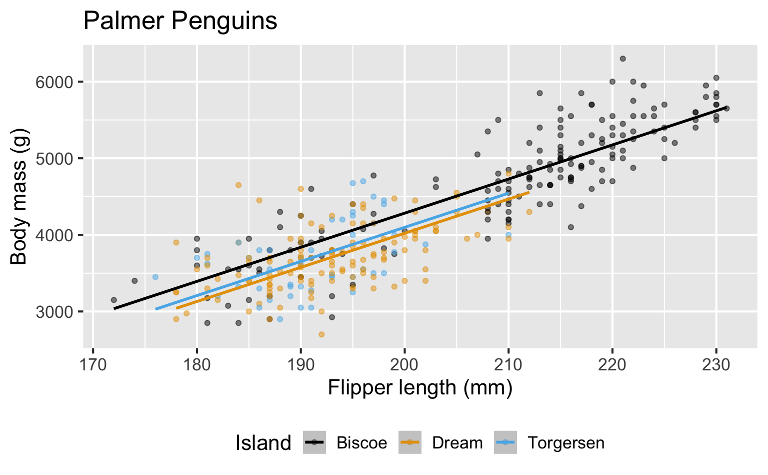
Recap: multiple linear regression
Numerical outcome, numerical and categorical predictors:
A binary outcome
\[ y = \begin{cases} 1 & &&\text{eg. Yes, Win, True, Heads, Success}\\ 0 & &&\text{eg. No, Lose, False, Tails, Failure}. \end{cases} \]
Example: Is it cancer or not?
\(\mathbf{x}\): features in a medical image
\[ y = \begin{cases} 1 & \text{it's cancer}\\ 0 & \text{it's healthy} \end{cases} \]

Example: Will they default?
\(\mathbf{x}\): financial and demographic info about a loan applicant
\[ y = \begin{cases} 1 & \text{applicant is at risk of defaulting on loan}\\ 0 & \text{applicant is safe} \end{cases} \]

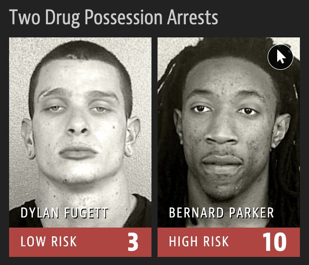
Example: Will they reoffend?
\(\mathbf{x}\): info about a criminal suspect and their case
\[ y = \begin{cases} 1 & \text{suspect is at risk of re-offending pre-trial}\\ 0 & \text{suspect is safe} \end{cases} \]

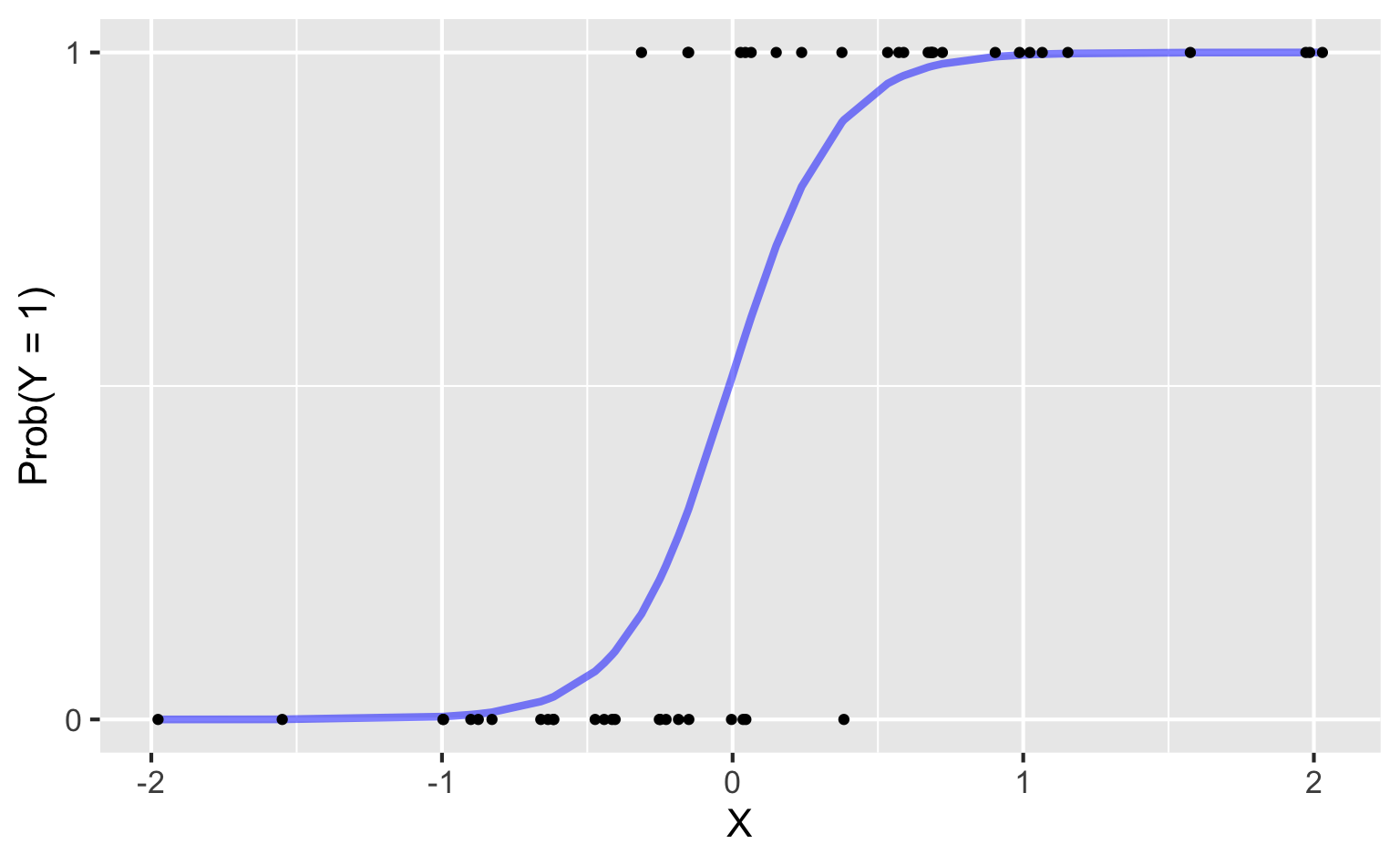
How do we model this type of data?
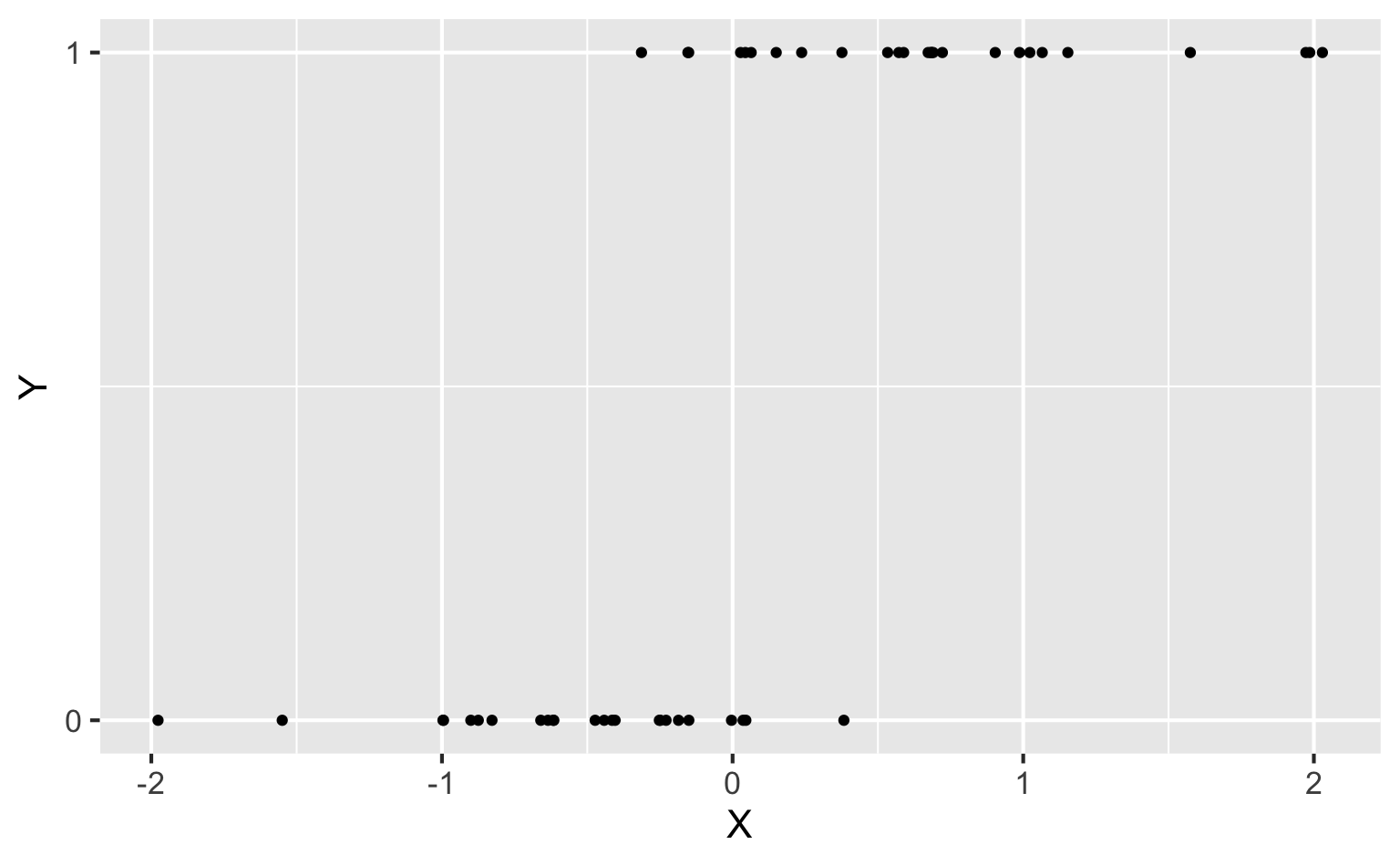
Straight line of best fit is a little silly
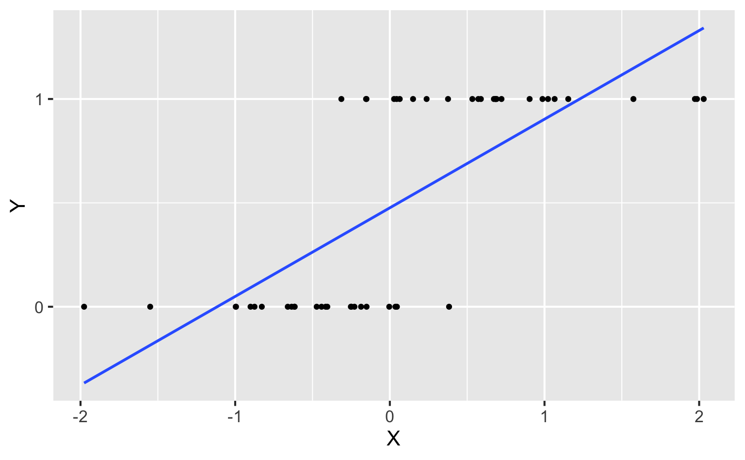
Instead: S-curve of best fit
Instead of modeling \(y\) directly, we model the probability that \(y=1\):

- “Given new email, what’s the probability that it’s spam?”
- “Given new image, what’s the probability that it’s cancer?”
- “Given new loan application, what’s the probability that applicant defaults?”
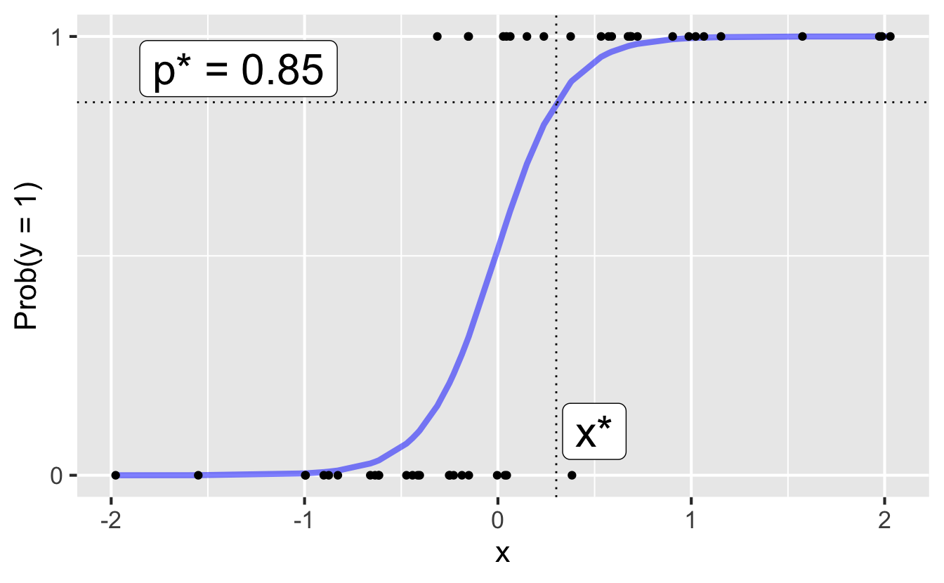
Step 1: Pick a threshold
Select a number \(0 < p^* < 1\):
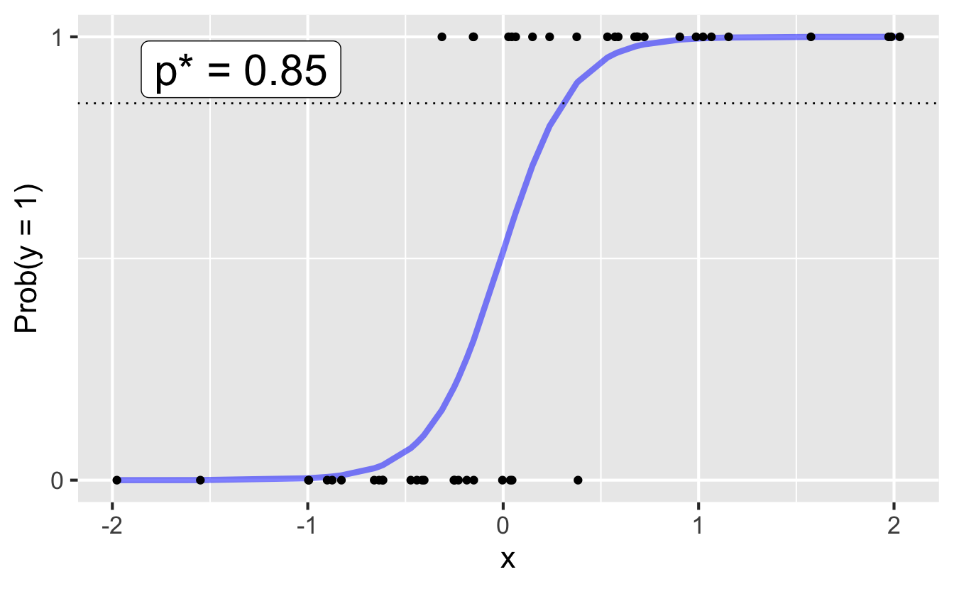
- if \(\text{Prob}(y=1)\leq p^*\), then predict \(\widehat{y}=0\)
- if \(\text{Prob}(y=1)> p^*\), then predict \(\widehat{y}=1\)
Step 2: Find the decision boundary
Solve for the x-value that matches the threshold:
- if \(\text{Prob}(y=1)\leq p^*\), then predict \(\widehat{y}=0\)
- if \(\text{Prob}(y=1)> p^*\), then predict \(\widehat{y}=1\)
Step 3: Classify a new arrival
A new data point is observed up with \(x_{\text{new}}\). Which side of the boundary is it on?
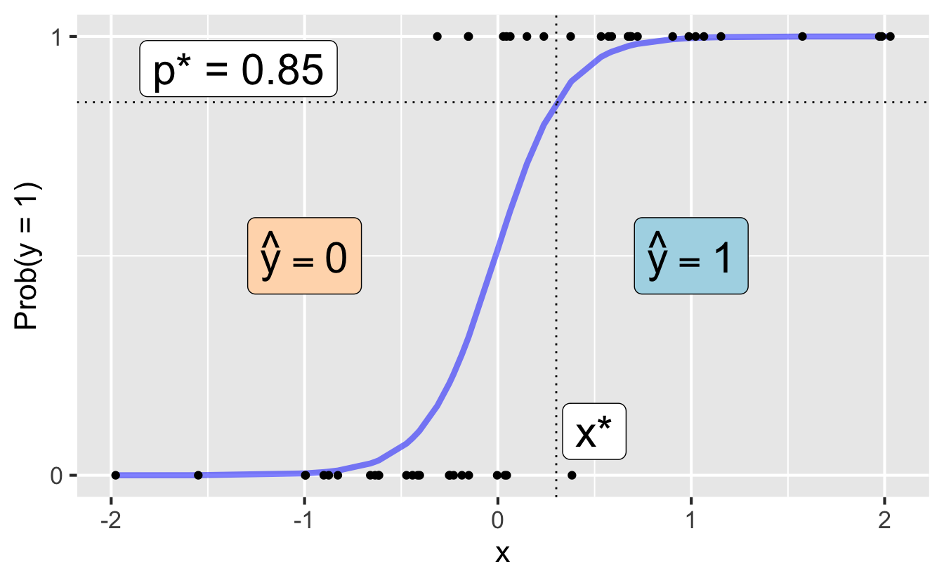
- if \(x_{\text{new}} \leq x^\star\), then \(\text{Prob}(y=1)\leq p^*\), so predict \(\widehat{y}=0\) for the new observation
- if \(x_{\text{new}} > x^\star\), then \(\text{Prob}(y=1)> p^*\), so predict \(\widehat{y}=1\) for the new observation
Let’s change the threshold
A new data point is observed with \(x_{\text{new}}\). Which side of the boundary are they on?
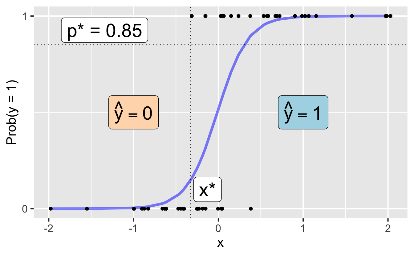
- if \(x_{\text{new}} \leq x^\star\), then \(\text{Prob}(y=1)\leq p^*\), so predict \(\widehat{y}=0\) for the new observation
- if \(x_{\text{new}} > x^\star\), then \(\text{Prob}(y=1)> p^*\), so predict \(\widehat{y}=1\) for the new observation
Nothing special about one predictor…
Two numerical predictors and one binary outcome:
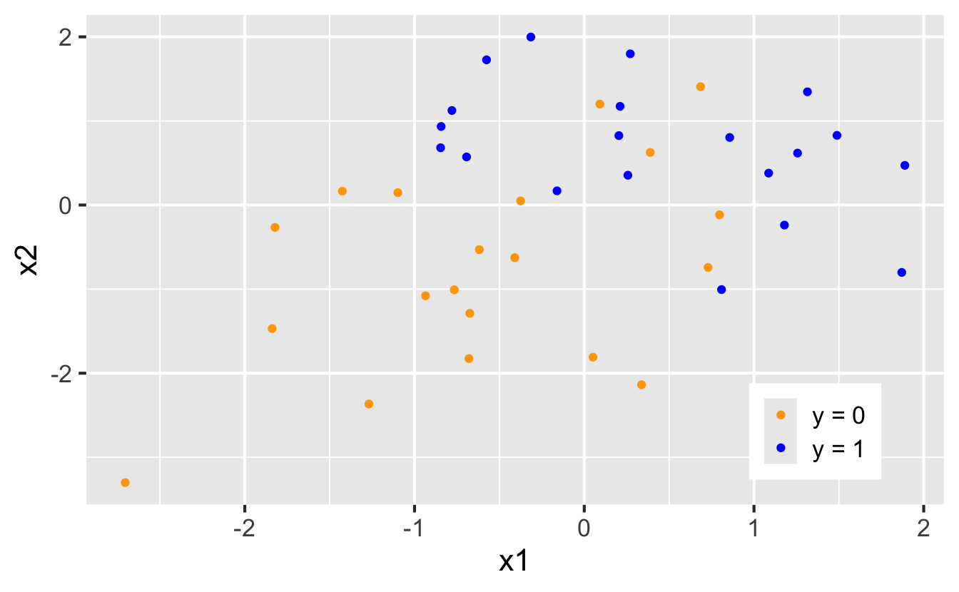
Decision boundary, again
It’s linear! Consider two numerical predictors:
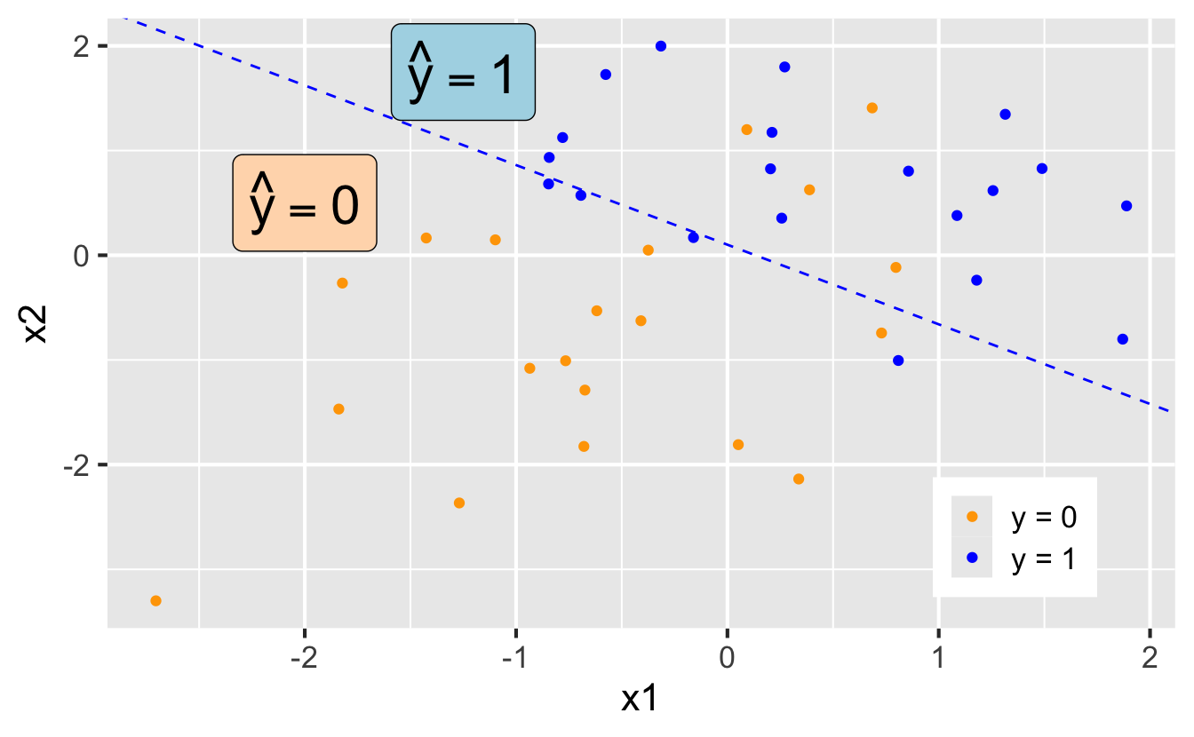
- if new \((x_1,\,x_2)\) below, \(\text{Prob}(y=1)\leq p^*\). Predict \(\widehat{y}=0\) for the new observation
- if new \((x_1,\,x_2)\) above, \(\text{Prob}(y=1)> p^*\). Predict \(\widehat{y}=1\) for the new observation