Bootstrapping

Modeling and inference

Data Science with R

Setup

Packages

tidyverse for data wrangling and visualization
tidymodels for modeling

library(tidyverse)
library(tidymodels)

Data: Rent in Edinburgh

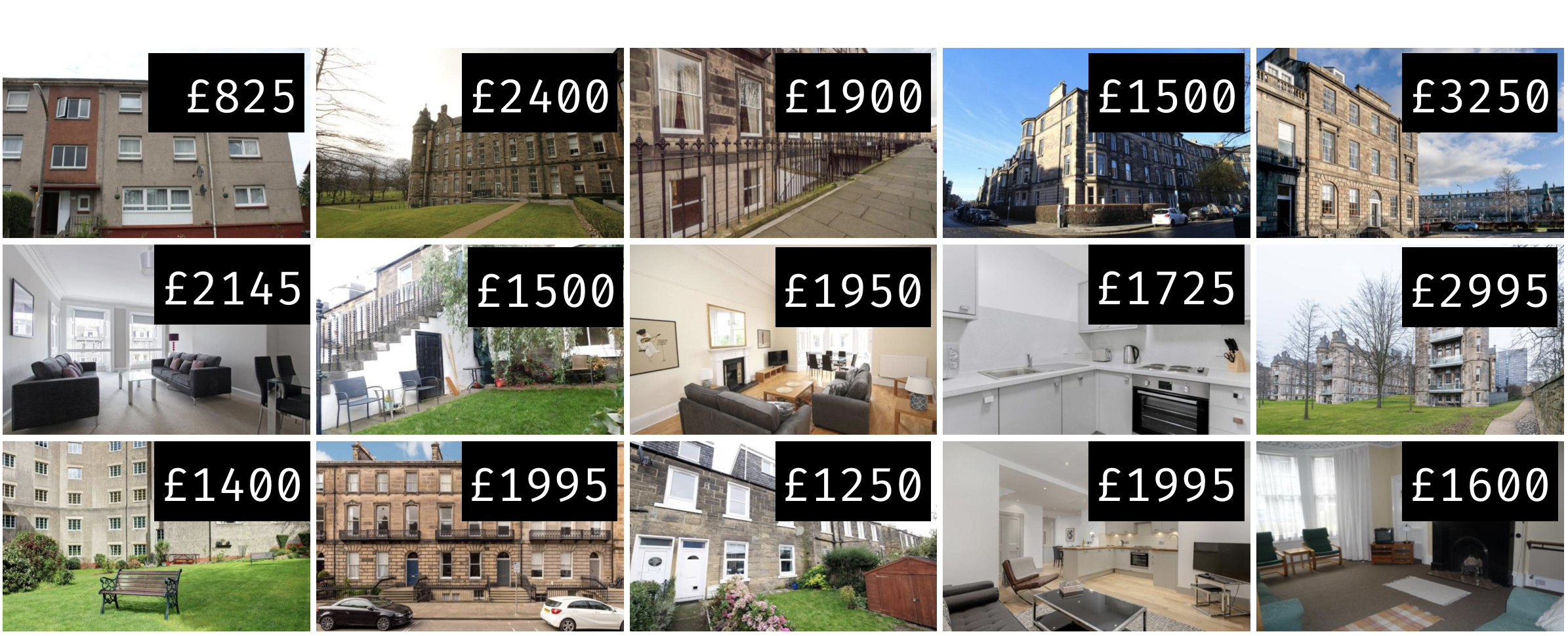
Fifteen 3 bedroom flats in Edinburgh, Scotland were randomly selected on rightmove.co.uk.

flat_id; rent; title; address
flat_01; 825 ; 3 bedroom apartment to rent; Burnhead Grove, Edinburgh, Midlothian, EH16
flat_02; 2400; 3 bedroom flat to rent; Simpson Loan, Quartermile, Edinburgh, EH3
flat_03; 1900; 3 bedroom flat to rent; FETTES ROW, NEW TOWN, EH3 6SE
flat_04; 1500; 3 bedroom apartment to rent; Eyre Crescent, Edinburgh, Midlothian
flat_05; 3250; 3 bedroom flat to rent; Walker Street, Edinburgh
flat_06; 2145; 3 bedroom flat to rent; George Street, City Centre, Edinburgh, EH2
flat_07; 1500; 3 bedroom flat to rent; Waverley Place , Edinburgh EH7 5SA
flat_08; 1950; 3 bedroom flat to rent; Drumsheugh Place, Edinburgh
flat_09; 1725; 3 bedroom flat to rent; Crighton Place, Leith, Edinburgh, EH7
flat_10; 2995; 3 bedroom flat to rent; Simpson Loan, Meadows, Edinburgh, EH3
flat_11; 1400; 3 bedroom flat to rent; 42, Learmonth Court, Edinburgh EH4 1PD
flat_12; 1995; 3 bedroom apartment to rent; Chester Street, Edinburgh, Midlothian
flat_13; 1250; 3 bedroom duplex to rent; Elmwood Terrace, Lochend, Edinburgh, EH6
flat_14; 1995; 3 bedroom apartment to rent; Great King Street, Edinburgh, EH3
flat_15; 1600; 3 bedroom ground floor flat to rent; Roseneath Terrace,Edinburgh,EH9

Load data

edi_3br <- read_csv2("data/edi-3br.csv") # ; separated
edi_3br

# A tibble: 15 × 4
   flat_id  rent title                               address
   <chr>   <dbl> <chr>                               <chr>  
 1 flat_01   825 3 bedroom apartment to rent         Burnhe…
 2 flat_02  2400 3 bedroom flat to rent              Simpso…
 3 flat_03  1900 3 bedroom flat to rent              FETTES…
 4 flat_04  1500 3 bedroom apartment to rent         Eyre C…
 5 flat_05  3250 3 bedroom flat to rent              Walker…
 6 flat_06  2145 3 bedroom flat to rent              George…
 7 flat_07  1500 3 bedroom flat to rent              Waverl…
 8 flat_08  1950 3 bedroom flat to rent              Drumsh…
 9 flat_09  1725 3 bedroom flat to rent              Cright…
10 flat_10  2995 3 bedroom flat to rent              Simpso…
11 flat_11  1400 3 bedroom flat to rent              42, Le…
12 flat_12  1995 3 bedroom apartment to rent         Cheste…
13 flat_13  1250 3 bedroom duplex to rent            Elmwoo…
14 flat_14  1995 3 bedroom apartment to rent         Great …
15 flat_15  1600 3 bedroom ground floor flat to rent Rosene…

Observed sample

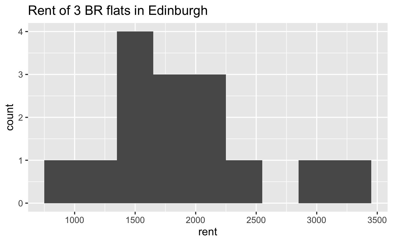
Observed sample

Sample mean ≈ £1895

Bootstrap population

Generated assuming there are more flats like the ones in the observed sample… Population mean = ?

Bootstrapping scheme

Take a bootstrap sample - a random sample taken with replacement from the original sample, of the same size as the original sample
Calculate the bootstrap statistic - a statistic such as mean, median, proportion, slope, etc. computed on the bootstrap samples
Repeat steps (1) and (2) many times to create a bootstrap distribution - a distribution of bootstrap statistics
Calculate the bounds of the XX% confidence interval as the middle XX% of the bootstrap distribution

Bootstrapping with tidymodels

Set a seed

set.seed(12345)

Specify the variable of interest

set.seed(12345)

edi_3br |>
  specify(response = rent)

Response: rent (numeric)
# A tibble: 15 × 1
    rent
   <dbl>
 1   825
 2  2400
 3  1900
 4  1500
 5  3250
 6  2145
 7  1500
 8  1950
 9  1725
10  2995
11  1400
12  1995
13  1250
14  1995
15  1600

Generate 15000 bootstrap samples

set.seed(12345)

edi_3br |>
  specify(response = rent) |>
  generate(reps = 15000, type = "bootstrap")

Response: rent (numeric)
# A tibble: 225,000 × 2
# Groups:   replicate [15,000]
   replicate  rent
       <int> <dbl>
 1         1  1995
 2         1  1900
 3         1  2995
 4         1  1995
 5         1  1950
 6         1  2995
 7         1  1250
 8         1  1400
 9         1  1950
10         1  2400
# ℹ 224,990 more rows

Calculate the mean of each bootstrap sample

set.seed(12345)

edi_3br |>
  specify(response = rent) |>
  generate(reps = 15000, type = "bootstrap") |>
  calculate(stat = "mean")

Response: rent (numeric)
# A tibble: 15,000 × 2
   replicate  stat
       <int> <dbl>
 1         1 2001 
 2         2 1886 
 3         3 1799.
 4         4 1968.
 5         5 1789 
 6         6 2018 
 7         7 1995.
 8         8 1867.
 9         9 2042 
10        10 1776.
# ℹ 14,990 more rows

Save resulting bootstrap distribution

set.seed(12345)

boot_dist <- edi_3br |>
  specify(response = rent) |>
  generate(reps = 15000, type = "bootstrap") |>
  calculate(stat = "mean")

The bootstrap sample

How many observations are there in boot_dist? What does each observation represent?

boot_dist

Response: rent (numeric)
# A tibble: 15,000 × 2
   replicate  stat
       <int> <dbl>
 1         1 2001 
 2         2 1886 
 3         3 1799.
 4         4 1968.
 5         5 1789 
 6         6 2018 
 7         7 1995.
 8         8 1867.
 9         9 2042 
10        10 1776.
# ℹ 14,990 more rows

Visualize the bootstrap distribution

visualize(boot_dist)

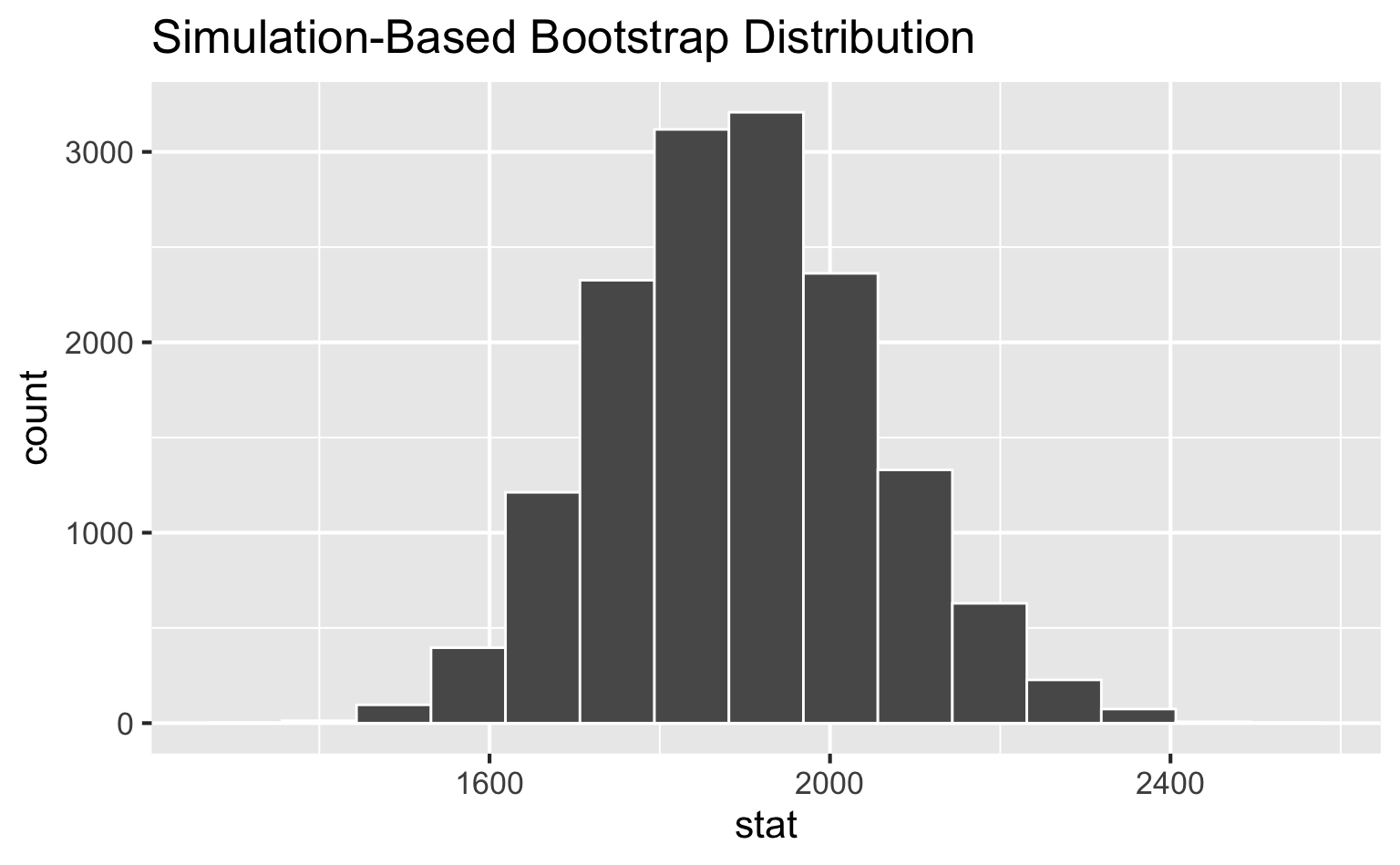
Calculate the confidence interval

A 95% confidence interval is bounded by the middle 95% of the bootstrap distribution.

ci_95 <- get_ci(
  boot_dist,
  level = 0.95
)
ci_95

# A tibble: 1 × 2
  lower_ci upper_ci
     <dbl>    <dbl>
1     1601    2216.

Visualize the confidence interval

visualize(boot_dist) +
  shade_ci(ci_95)

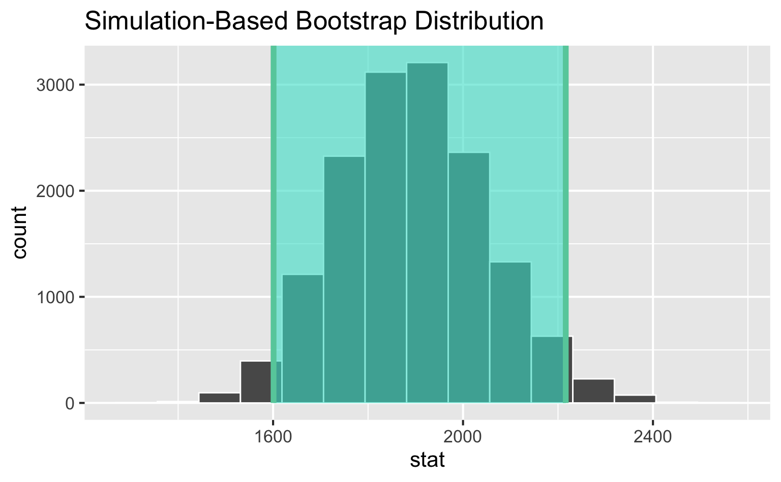
Interpret the confidence interval

What do the bounds og the confidence interval for the mean rent of three bedroom flats in Edinburgh (1601, 2216) represent?

95% of the time the mean rent of three bedroom flats in this sample is between £1601 and £2216.
95% of all three bedroom flats in Edinburgh have rents between £1601 and £2216.
We are 95% confident that the mean rent of all three bedroom flats is between £1601 and £2216.
We are 95% confident that the mean rent of three bedroom flats in this sample is between £1601 and £2216.

Accuracy vs. precision

Confidence level

We are 95% confident that …

Suppose we took many samples from the original population and built a 95% confidence interval based on each sample.
Then about 95% of those intervals would contain the true population parameter.

Commonly used confidence levels

Which line (orange dash/dot, blue dash, green dot) represents which confidence level?

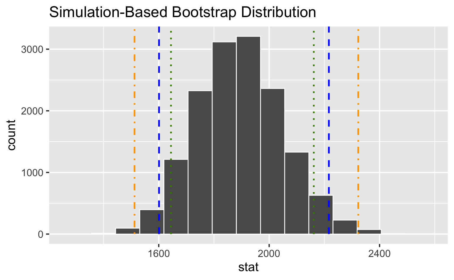
Precision vs. accuracy

If we want to be very certain that we capture the population parameter, should we use a wider or a narrower interval? What drawbacks are associated with using a wider interval?

How can we get best of both worlds – high precision and high accuracy?

Changing confidence level

How would you modify the following code to calculate a 90% confidence interval? How would you modify it for a 99% confidence interval?

set.seed(12345)

edi_3br |>
  specify(response = rent) |>
  generate(reps = 15000, type = "bootstrap") |>
  calculate(stat = "mean") |>
  get_ci(level = 0.95)

# A tibble: 1 × 2
  lower_ci upper_ci
     <dbl>    <dbl>
1     1601    2216.

Changing confidence level

How would you modify the following code to calculate a 90% confidence interval? How would you modify it for a 99% confidence interval?

set.seed(12345)

edi_3br |>
  specify(response = rent) |>
  generate(reps = 15000, type = "bootstrap") |>
  calculate(stat = "mean") |>
  get_ci(level = 0.90)

# A tibble: 1 × 2
  lower_ci upper_ci
     <dbl>    <dbl>
1    1644.    2162.

Changing confidence level

How would you modify the following code to calculate a 90% confidence interval? How would you modify it for a 99% confidence interval?

set.seed(12345)

edi_3br |>
  specify(response = rent) |>
  generate(reps = 15000, type = "bootstrap") |>
  calculate(stat = "mean") |>
  get_ci(level = 0.99)

# A tibble: 1 × 2
  lower_ci upper_ci
     <dbl>    <dbl>
1    1512.    2323.

Recap

Sample statistic \(\ne\) population parameter, but if the sample is good, it can be a good estimate
We report the estimate with a confidence interval, and the width of this interval depends on the variability of sample statistics from different samples from the population
Since we can’t continue sampling from the population, we bootstrap from the one sample we have to estimate sampling variability
We can do this for any sample statistic:
- For a mean: calculate(stat = "mean")
- For a median: calculate(stat = "median")
- … and so on